ggtextExtra
- Part 000. Abstract
- Part 00. Proposal
- Part 0. Lay out package infrastructure
- Part 00 Explore ggplot object internals
- Part I. Work out functionality 🚧 ✅
- Further bundling
- Issues/Notes:
- Part II. Packaging and documentation
- Bit 8: Compile readme
- Bit 9: Push to github
- Bit 10: listen and iterate
- Appendix: Reports, Environment
When participants were shown visualizations with titles during encoding, the titles were fixated 59% of the time. Correspondingly, during the recall phase of the experiment, titles were the element most likely to be described if present (see Fig. 8). When presented visualizations with titles, 46% of the time the participants described the contents, or rewording, of the title. - Beyond Memorability: Visualization Recognition and Recall
Across all textual elements, the title is among the most important. A good or a bad title can sometimes make all of the difference between a visualization that is recalled correctly from one that is not - Beyond Memorability: Visualization Recognition and Recall https://vcg.seas.harvard.edu/files/pfister/files/infovis_submission251-camera.pdf
Part 000. Abstract
ggplot2 users sometimes forego a color or fill legend, instead coloring the text of categories in a title or annotation as they make mention of them using ggtext.
But the process for doing this, I believe, can be somewhat tedious and error prone, because you have to type your own html color tags. The color tags also might make source composed title text less readable.
I admire these plots, but maybe have made them once because they require some stamina and focus to choreograph the colored text coordination.
Below we ‘crack open ggplot2 internals’ to try to streamline this process. Our objective is that text coloring automatically matches whatever ggplot2 is doing with color and fill scales.
Part 00. Proposal
This repo proposes the {ggtextExtra} package. 🦄
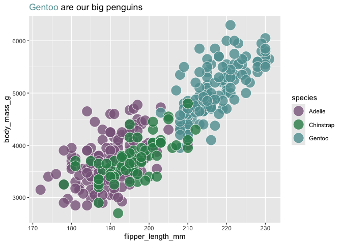
The goal of {ggtextExtra} is to make matching colors text written via ggtext moves to ggplot2 layers (geoms that are filled or colored).
There’s just one function that’s worked out so far (matching fill color for title), but I think it’s a useful one and could be easily extended to other areas (geom_textbox, color).
Without the package, we can do something like the following 🏋:
library(tidyverse)
#> ── Attaching core tidyverse packages ──────────────────────── tidyverse 2.0.0 ──
#> ✔ dplyr     1.1.4     ✔ readr     2.1.5
#> ✔ forcats   1.0.0     ✔ stringr   1.5.1
#> ✔ ggplot2   3.5.1     ✔ tibble    3.2.1
#> ✔ lubridate 1.9.3     ✔ tidyr     1.3.1
#> ✔ purrr     1.0.2
#> ── Conflicts ────────────────────────────────────────── tidyverse_conflicts() ──
#> ✖ dplyr::filter() masks stats::filter()
#> ✖ dplyr::lag()    masks stats::lag()
#> ℹ Use the conflicted package (<http://conflicted.r-lib.org/>) to force all conflicts to become errors

palmerpenguins::penguins  |>
 ggplot(aes(flipper_length_mm, body_mass_g,
             fill = species)) +
  geom_point(size = 7, alpha = .8, shape = 21, color = "white") +
  scale_fill_manual(values = c("plum4", "seagreen", "cadetblue")) +
  labs(title = "<span style = 'color: cadetblue;'>Gentoo</span> are our big penguins") +
  theme(plot.title = ggtext::element_markdown())
#> Warning: Removed 2 rows containing missing values or values outside the scale range
#> (`geom_point()`).
An approach that automates the coordination a bit more can be found here. https://albert-rapp.de/posts/16_html_css_for_r/16_html_css_for_r
library(tidyverse)

colors <- thematic::okabe_ito(2)
names(colors) <- c('male', 'female')

palmerpenguins::penguins |>
  filter(!is.na(sex)) |>
  ggplot(aes(bill_length_mm, flipper_length_mm, fill = sex)) +
  geom_point(size = 3, alpha = 0.75, col = 'black', shape = 21) +
  labs(
    x = 'Bill length (in mm)',
    y = 'Flipper length (in mm)',
    title = glue::glue('Measurements of <span style="color:{colors["male"]}">**male**</span> and <span style=color:{colors["female"]}>**female**</span> penguins')
  ) +
  scale_fill_manual(values = colors)
But this requires a bit more in the way of presteps and writing text in the html tags; these tags also might make the readability of the title even more challenging.
With the {ggtextExtra} package, we’ll live in a different world (🦄 🦄 🦄) where the task a little more automatic:
Proposed API will:
- Build a ggplot in the usual way. I.e. do whatever you like with color/fill mapping to categories
- apply a function to that automatically checks the colors used to represent categories and applies those in the title where the categories appear. (via ggtext::element_markdown).
What that would look like in code:
my_title <- "The **setosa** irises has the largest average sapel widths <br>and then comes **virginica** irises while<br>**versicolor** has the shortest sapel width"

palmerpenguins::penguins  |>
 ggplot(aes(flipper_length_mm, body_mass_g,
             fill = species)) +
  geom_point(shape = 21,
             color = "white", size = 8, alpha = .9) +
  scale_fill_viridis_d(end = .8, begin = .2) +
  labs(title = my_title) +
  theme(plot.title = ggtext::element_markdown())

use_fill_scale_in_title_words(plot = last_plot()) +
  guides(fill = "none")
Part 0. Lay out package infrastructure
devtools::create(".")
Part 00 Explore ggplot object internals
Now let’s ‘crack into ggplot2 internals’ to see if we can get to a match between categories and colors programmatically.
First, we’ll look at the colors actually rendered in the layer data of
the plot using layer_data. These are often (always?) stored as hex
colors which will definitely work in html/markdown context, whereas you
have to be a little careful with some R named colors not working at all
in html.
grab fill color and associated group with layer_data
First, we’ll use layer_data to grab fill and group.
plot <- last_plot()

fill_values_df <- layer_data(plot, i = 1) %>%  .[,c("fill", "group")] |> distinct()
fill_values_df
#>        fill group
#> 1     plum4     1
#> 2 cadetblue     3
#> 3  seagreen     2
grab the name of the variable that’s mapped to fill
Then we’ll grab the name of the variable that’s mapped to fill. This seems a little weird, but seems to works. Open to different approaches that might be more robust!
fill_var_name <- plot$mapping$fill |> capture.output() %>% .[2] %>% str_extract("\\^.+") %>% str_remove("\\^")
fill_var_name
#> [1] "species"
grab the categories in the mapped variable
Then we can grab the actual vector of data that’s being represented by
fill color - the plot$data slot. We put this in a dataframe/tibble,
and then used distinct to get a one-to-one category-group table.
fill_var_df <- plot$data[fill_var_name] %>% distinct()
fill_var_df
#> # A tibble: 3 × 1
#>   species
#>   <fct>
#> 1 Adelie
#> 2 Gentoo
#> 3 Chinstrap
names(fill_var_df) <- "fill_var"
fill_var_df <- mutate(fill_var_df, group = as.numeric(fill_var))
fill_var_df
#> # A tibble: 3 × 2
#>   fill_var  group
#>   <fct>     <dbl>
#> 1 Adelie        1
#> 2 Gentoo        3
#> 3 Chinstrap     2
create a color-category crosswalk
Then we join our colors and categories by group, and have a color-category one-to-one table. And then we can prepare an html statement that will make the category colorful when rendered by ggtext functionality.
left_join(fill_values_df, fill_var_df, by = join_by(group)) %>%
  mutate(html_replacements =
           paste0("<span style = 'color: ", fill,
                         "'>", fill_var, "</span>") )
#>        fill group  fill_var                                html_replacements
#> 1     plum4     1    Adelie       <span style = 'color: plum4'>Adelie</span>
#> 2 cadetblue     3    Gentoo   <span style = 'color: cadetblue'>Gentoo</span>
#> 3  seagreen     2 Chinstrap <span style = 'color: seagreen'>Chinstrap</span>
Part I. Work out functionality 🚧 ✅
The above looks pretty promising so let’s put this in a function. The function will let us go straight from a ggplot2 plot object to a category-color-htmlreplcement data frame.
grab_fill_info <- function(plot = last_plot(), i = NULL){

  if(is.null(i)){i <- length(plot$layers)}

fill_values_df <- ggplot2::layer_data(plot, i = i) %>%
  .[,c("fill", "group")] |>
  dplyr::distinct()

fill_var_name <- plot$mapping$fill |>
  capture.output() %>% .[2] %>%
  stringr::str_extract("\\^.+") %>%
  stringr::str_remove("\\^")

fill_var_df <- plot$data[,fill_var_name] |>
  dplyr::distinct()

names(fill_var_df) <- "fill_var"

fill_var_df <- fill_var_df |> mutate(group = as.numeric(as.factor(fill_var)))


dplyr::left_join(fill_values_df,
                 fill_var_df,
                 by = dplyr::join_by(group)) %>%
  dplyr::mutate(html_replacements =
                  paste0("<span style = 'color: ",
                         .data$fill,
                         "'>",
                         .data$fill_var,
                         "</span></strong>") ) %>%
  ggplot2::remove_missing()  # where category is NA

}
We can test this out with the plot we saved before:
grab_fill_info(plot = plot)
#>        fill group  fill_var
#> 1     plum4     1    Adelie
#> 2 cadetblue     3    Gentoo
#> 3  seagreen     2 Chinstrap
#>                                           html_replacements
#> 1       <span style = 'color: plum4'>Adelie</span></strong>
#> 2   <span style = 'color: cadetblue'>Gentoo</span></strong>
#> 3 <span style = 'color: seagreen'>Chinstrap</span></strong>
A first cut at find-replace to add html color tags automatically to a string
And then we’ll use the data frame output, to make replacements in a string, adding the html tags. We’ll just get it done with a for loop. One danger, that I’m leaving for later, is that you might have a categories like ‘anana’ (this means pineapple in Portuguese and maybe some other languages) and ‘banana’ (this means banana in Portuguese and maybe some other languages). In this case, you’ll have a bad result given the current implementation. (Anana has an acent on the final syllable in Portuguese you might actually be saved!) male/female is the same problem - but not as nice of a tangent.
fill_df <- grab_fill_info(plot)

for(i in 1:nrow(fill_df)){

  start <- "Gentoo have the longest average flippers"

  start <- start |> stringr::str_replace(fill_df$fill_var[i] %>% as.character(), fill_df$html_replacements[i])

start %>% print()

}
#> [1] "Gentoo have the longest average flippers"
#> [1] "<span style = 'color: cadetblue'>Gentoo</span></strong> have the longest average flippers"
#> [1] "Gentoo have the longest average flippers"
Let’s put the for loop in a function:
auto_color_html <- function(x, fill_df ){

 for(i in 1:nrow(fill_df)){

  x <- x |> stringr::str_replace(fill_df$fill_var[i] %>% as.character, fill_df$html_replacements[i])

 }

  x

}
Test it out…
auto_color_html("The Gentoo is a cool penguin", grab_fill_info(plot))
#> [1] "The <span style = 'color: cadetblue'>Gentoo</span></strong> is a cool penguin"
Try out constituent functions w/ a fresh plot
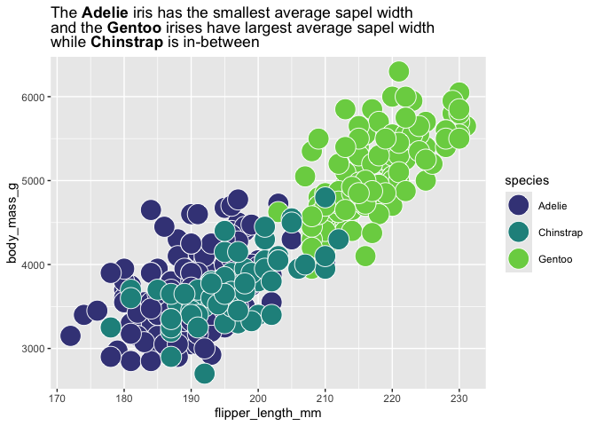
Now let’s use our functions with a fresh plot, q.
palmerpenguins::penguins  |>
 ggplot(aes(flipper_length_mm, body_mass_g,
             fill = species)) +
  geom_point(shape = 21, color = "white", size = 8) +
  scale_fill_viridis_d(end = .8, begin = .2) +
  labs(title = "The **Adelie** iris has the smallest average sapel width<br>and the **Gentoo** irises have largest average sapel width<br>
       while **Chinstrap** is in-between") +
  theme(plot.title = ggtext::element_markdown())
#> Warning: Removed 2 rows containing missing values or values outside the scale range
#> (`geom_point()`).
q <- last_plot()

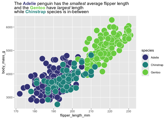
q_fill_df <- grab_fill_info(q)

colorful_title <- "The **Adelie** penguin has the *smallest* average flipper length<br>and the **Gentoo** have *largest* length<br> while **Chinstrap** species is in-between" |>
        auto_color_html(q_fill_df)

q +
  labs(title = colorful_title)  #overwriting title
#> Warning: Removed 2 rows containing missing values or values outside the scale range
#> (`geom_point()`).
Further bundling
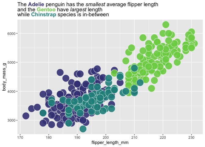
Looks good. What if we wrap everything, and just replace the title with an html color-tagged version.
use_fill_scale_in_title_words <- function(plot, i = NULL){

  out <- plot

  if(!is.null(i)){i <- length(plot$layers)}  # looks at last layer for fill colors

  plot_fill_df <- grab_fill_info(plot, i = i)

  out$labels$title <- out$labels$title |>
        auto_color_html(plot_fill_df)

  return(out)

}
Try it out starting fresh.
my_title <- "The **Adelie** penguin has the *smallest* average flipper length<br>and the **Gentoo** have *largest* length<br> while **Chinstrap** species is in-between"

palmerpenguins::penguins |>
 ggplot() +
  aes(x = flipper_length_mm,
      y = body_mass_g,
      fill = species) +
  geom_point(shape = 21,
             color = "white", size = 8, alpha = .9) +
  scale_fill_viridis_d(end = .8, begin = .2) +
  labs(title = my_title) +
  theme(plot.title = ggtext::element_markdown())
#> Warning: Removed 2 rows containing missing values or values outside the scale range
#> (`geom_point()`).

use_fill_scale_in_title_words(plot = last_plot()) +
  guides(fill = "none")
#> Warning: Removed 2 rows containing missing values or values outside the scale range
#> (`geom_point()`).
# Option 2: Read directly from GitHub

wwbi_data <- readr::read_csv('https://raw.githubusercontent.com/rfordatascience/tidytuesday/master/data/2024/2024-04-30/wwbi_data.csv')
#> Rows: 141985 Columns: 4
#> ── Column specification ────────────────────────────────────────────────────────
#> Delimiter: ","
#> chr (2): country_code, indicator_code
#> dbl (2): year, value
#>
#> ℹ Use `spec()` to retrieve the full column specification for this data.
#> ℹ Specify the column types or set `show_col_types = FALSE` to quiet this message.
wwbi_series <- readr::read_csv('https://raw.githubusercontent.com/rfordatascience/tidytuesday/master/data/2024/2024-04-30/wwbi_series.csv')
#> Rows: 302 Columns: 2
#> ── Column specification ────────────────────────────────────────────────────────
#> Delimiter: ","
#> chr (2): indicator_code, indicator_name
#>
#> ℹ Use `spec()` to retrieve the full column specification for this data.
#> ℹ Specify the column types or set `show_col_types = FALSE` to quiet this message.
wwbi_country <- readr::read_csv('https://raw.githubusercontent.com/rfordatascience/tidytuesday/master/data/2024/2024-04-30/wwbi_country.csv')
#> Rows: 202 Columns: 29
#> ── Column specification ────────────────────────────────────────────────────────
#> Delimiter: ","
#> chr (21): country_code, short_name, table_name, long_name, x2_alpha_code, cu...
#> dbl  (7): national_accounts_base_year, national_accounts_reference_year, sys...
#> lgl  (1): vital_registration_complete
#>
#> ℹ Use `spec()` to retrieve the full column specification for this data.
#> ℹ Specify the column types or set `show_col_types = FALSE` to quiet this message.

head(wwbi_data)
#> # A tibble: 6 × 4
#>   country_code indicator_code     year value
#>   <chr>        <chr>             <dbl> <dbl>
#> 1 AFG          BI.WAG.PRVS.FM.SM  2007 1.11
#> 2 AFG          BI.WAG.PRVS.FM.SM  2013 0.649
#> 3 AFG          BI.WAG.PRVS.FM.MD  2007 0.533
#> 4 AFG          BI.WAG.PRVS.FM.MD  2013 0.433
#> 5 AFG          BI.WAG.PUBS.FM.SM  2007 0.858
#> 6 AFG          BI.WAG.PUBS.FM.SM  2013 0.661
head(wwbi_series)
#> # A tibble: 6 × 2
#>   indicator_code       indicator_name
#>   <chr>                <chr>
#> 1 BI.EMP.FRML.CA.PB.ZS Core Public Administration workers, as a share of public…
#> 2 BI.EMP.FRML.ED.PB.ZS Education workers, as a share of public formal employees
#> 3 BI.EMP.FRML.HE.PB.ZS Health workers, as a share of public formal employees
#> 4 BI.EMP.FRML.MW.PB.ZS Medical workers, as a share of public formal employees
#> 5 BI.EMP.FRML.PB.ED.ZS Public sector employment, as a share of formal employmen…
#> 6 BI.EMP.FRML.PB.HE.ZS Public sector employment, as a share of formal employmen…
head(wwbi_country)
#> # A tibble: 6 × 29
#>   country_code short_name       table_name long_name x2_alpha_code currency_unit
#>   <chr>        <chr>            <chr>      <chr>     <chr>         <chr>
#> 1 ABW          Aruba            Aruba      Aruba     AW            Aruban florin
#> 2 AFG          Afghanistan      Afghanist… Islamic … AF            Afghan afgha…
#> 3 AGO          Angola           Angola     People's… AO            Angolan kwan…
#> 4 AIA          Anguilla         Anguilla   Anguilla… <NA>          Eastern Cari…
#> 5 ALB          Albania          Albania    Republic… AL            Albanian lek
#> 6 ARE          United Arab Emi… United Ar… United A… AE            U.A.E. dirham
#> # ℹ 23 more variables: special_notes <chr>, region <chr>, income_group <chr>,
#> #   wb_2_code <chr>, national_accounts_base_year <dbl>,
#> #   national_accounts_reference_year <dbl>, sna_price_valuation <chr>,
#> #   lending_category <chr>, other_groups <chr>,
#> #   system_of_national_accounts <dbl>, balance_of_payments_manual_in_use <chr>,
#> #   external_debt_reporting_status <chr>, system_of_trade <chr>,
#> #   government_accounting_concept <chr>, …

wwbi_series %>%
  filter(indicator_code == "BI.EMP.PWRK.PB.HE.ZS") %>%
  .[2] ->
y_var

wwbi_data %>%
  filter(indicator_code == "BI.EMP.PWRK.PB.HE.ZS"    ) %>%
  left_join(wwbi_country) %>%
  filter(region == "Latin America & Caribbean") %>%
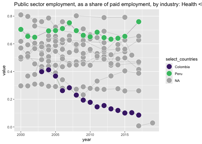
  mutate(is_select_country = short_name %in%
                                     c("Peru","Colombia")) %>%
  mutate(select_countries = ifelse(is_select_country,
                                   short_name, NA)) %>%
  arrange(is_select_country) %>%
  ggplot() +
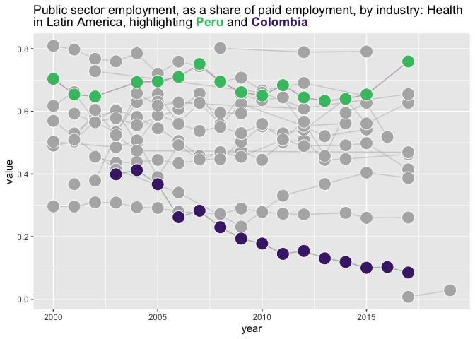
  labs(title = y_var %>%
         paste("<br>in Latin America, highlighting **Peru** and **Colombia**")) +
  aes(x = year, y = value, fill = select_countries, color = select_countries) +
  # geom_text(aes(label = country_code)) +
  geom_line(aes(group = country_code), alpha = .5) +
  geom_point(shape = 21, size = 6, color = "white") +
  scale_fill_manual(values = c("darkseagreen4", "plum4"), na.value = "grey70") +
  scale_color_manual(values = c("darkseagreen4", "plum4"), na.value = "grey70") +

  scale_fill_viridis_d(na.value = "grey70", end = .7, begin = .1) +
  # scale_fill_viridis_d() +  # no color..
  NULL
#> Joining with `by = join_by(country_code)`
#> Scale for fill is already present. Adding another scale for fill, which will
#> replace the existing scale.
use_fill_scale_in_title_words(last_plot()) +
  theme(plot.title = ggtext::element_markdown()) +
  guides(fill = "none", color = "none")
#> Warning: Removed 1 row containing missing values or values outside the scale
#> range.
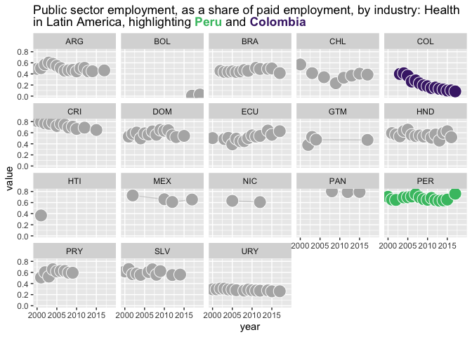
last_plot()+
  facet_wrap(~country_code)
#> `geom_line()`: Each group consists of only one observation.
#> ℹ Do you need to adjust the group aesthetic?
Issues/Notes:
- fill mapping should be globally declared
- data should be globally declared
- fill colors are taken from the last (top) layer unless i is changed.
- naive string replacement issue
Part II. Packaging and documentation
Phase 1. Minimal working package ✅
To build a minimal working package, 1) we’ll need to document dependencies 2) send functions to .R files in the R folder, 3) do a package check (this will A. Document our functions and B. this will help us identify problems - for example if we’ve failed to declare a dependency) and 4) install the package locally.
Then we’ll write up a quick advertisement for what our package is able to do in the ‘traditional readme’ section. This gives us a chance to test out the package.
### Bit 2a: in the function(s) you wrote above make sure dependencies to functions using '::' syntax to pkg functions
usethis::use_package("ggplot2") # Bit 2b: document dependencies, w hypothetical ggplot2
usethis::use_package("dplyr")
usethis::use_package("stringr")
usethis::use_package("tibble")
usethis::use_pipe()
knitrExtra::chunk_names_get()
#> It seems you are currently knitting a Rmd/Qmd file. The parsing of the file will be done in a new R session.
#>  [1] "unnamed-chunk-1"               "unnamed-chunk-2"
#>  [3] "unnamed-chunk-3"               "unnamed-chunk-4"
#>  [5] "unnamed-chunk-5"               "unnamed-chunk-6"
#>  [7] "unnamed-chunk-7"               "unnamed-chunk-8"
#>  [9] "grab_fill_info"                "unnamed-chunk-9"
#> [11] "unnamed-chunk-10"              "auto_color_html"
#> [13] "unnamed-chunk-11"              "unnamed-chunk-12"
#> [15] "use_fill_scale_in_title_words" "unnamed-chunk-13"
#> [17] "unnamed-chunk-14"              "unnamed-chunk-15"
#> [19] "unnamed-chunk-16"              "unnamed-chunk-17"
#> [21] "unnamed-chunk-18"              "unnamed-chunk-19"
#> [23] "unnamed-chunk-20"              "test_calc_times_two_works"
#> [25] "unnamed-chunk-21"              "unnamed-chunk-22"
#> [27] "unnamed-chunk-23"              "unnamed-chunk-24"
#> [29] "unnamed-chunk-25"              "unnamed-chunk-26"
# Bit 3: send the code chunk with function to R folder
knitrExtra:::chunk_to_r(chunk_name = "grab_fill_info")
#> It seems you are currently knitting a Rmd/Qmd file. The parsing of the file will be done in a new R session.
knitrExtra:::chunk_to_r(chunk_name = "auto_color_html")
#> It seems you are currently knitting a Rmd/Qmd file. The parsing of the file will be done in a new R session.
knitrExtra:::chunk_to_r(chunk_name = "use_fill_scale_in_title_words")
#> It seems you are currently knitting a Rmd/Qmd file. The parsing of the file will be done in a new R session.
# Bit 4: document functions and check that package is minimally viable
devtools::check(pkg = ".")

# Bit 5: install package locally
devtools::install(pkg = ".", upgrade = "never")
Bit 7. Write traditional README that uses built package (also serves as a test of build). ✅
The goal of the {ggtextExtra} package is to …
Install package with:
remotes::install_github("EvaMaeRey/ggtextExtra")
Once functions are exported you can remove go to two colons, and when things are are really finalized, then go without colons (and rearrange your readme…)
library(ggtextExtra)
#> Error in library(ggtextExtra): there is no package called 'ggtextExtra'
my_title <- "The **Adelie** penguin has the *smallest* average flipper length<br>and the **Gentoo** have *largest* length<br> while **Chinstrap** species is in-between"

palmerpenguins::penguins |>
 ggplot() +
  aes(x = flipper_length_mm,
      y = body_mass_g,
      fill = species) +
  geom_point(shape = 21,
             color = "white", size = 8, alpha = .9) +
  scale_fill_viridis_d(end = .8, begin = .2) +
  labs(title = my_title) +
  theme(plot.title = ggtext::element_markdown())
#> Warning: Removed 2 rows containing missing values or values outside the scale range
#> (`geom_point()`).
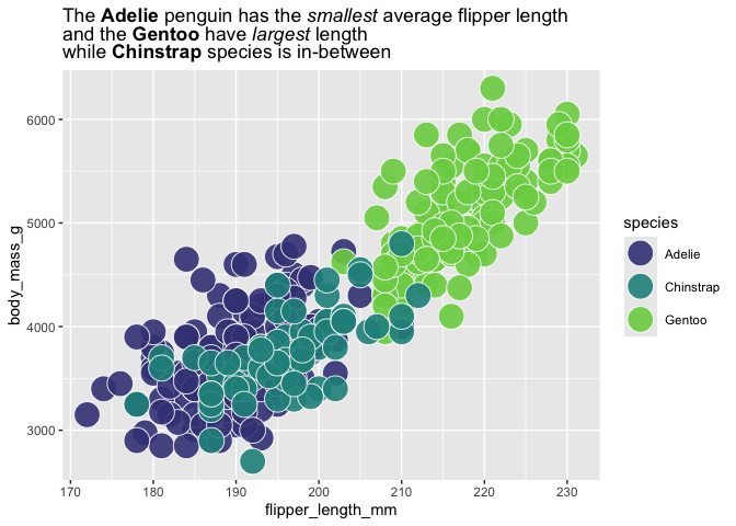
ggtextExtra:::use_fill_scale_in_title_words(plot = last_plot()) +
  guides(fill = "none")
#> Error in loadNamespace(x): there is no package called 'ggtextExtra'
Bit 8: Compile readme
Bit 9: Push to github
Bit 10: listen and iterate
Phase 3: Settling and testing 🚧
Bit A. Added a description and author information in the DESCRIPTION file 🚧
Bit B. Added roxygen skeleton for exported functions. 🚧
Bit D. Settle on examples. Put them in the roxygen skeleton and readme. 🚧
Bit C. Chosen a license? 🚧
usethis::use_mit_license()
Bit D. Use life-cycle badge
usethis::use_lifecycle_badge("experimental")
Bit E. Written formal tests of functions and save to test that folders 🚧
That would look like this…
library(testthat)

test_that("calc times 2 works", {
  expect_equal(times_two(4), 8)
  expect_equal(times_two(5), 10)

})
knitrExtra::chunk_to_tests_testthat("test_calc_times_two_works")
Bit F. Check again. Addressed notes, warnings and errors. 🚧
devtools::check(pkg = ".")
Phase 4. Promote to wider audience… 🚧
Bit A. Package website built? 🚧
Bit B. Package website deployed? 🚧
Phase 5: Harden/commit: Submit to CRAN/RUniverse 🚧
Appendix: Reports, Environment
Description file complete? 🚧
readLines("DESCRIPTION")
Environment 🚧
Here I just want to print the packages and the versions
all <- sessionInfo() |> print() |> capture.output()
all[11:17]
#> [1] ""
#> [2] "time zone: America/Denver"
#> [3] "tzcode source: internal"
#> [4] ""
#> [5] "attached base packages:"
#> [6] "[1] stats     graphics  grDevices utils     datasets  methods   base     "
#> [7] ""
devtools::check() report
devtools::check(pkg = ".")
Package directory file tree
fs::dir_tree(recurse = T)
#> .
#> ├── DESCRIPTION
#> ├── NAMESPACE
#> ├── R
#> │   ├── auto_color_html.R
#> │   ├── grab_fill_info.R
#> │   ├── use_fill_scale_in_title_words.R
#> │   └── utils-pipe.R
#> ├── README.Rmd
#> ├── README.md
#> ├── README_files
#> │   └── figure-gfm
#> │       ├── unnamed-chunk-11-1.png
#> │       ├── unnamed-chunk-11-2.png
#> │       ├── unnamed-chunk-12-1.png
#> │       ├── unnamed-chunk-12-2.png
#> │       ├── unnamed-chunk-13-1.png
#> │       ├── unnamed-chunk-13-2.png
#> │       ├── unnamed-chunk-13-3.png
#> │       ├── unnamed-chunk-14-1.png
#> │       ├── unnamed-chunk-14-2.png
#> │       ├── unnamed-chunk-14-3.png
#> │       ├── unnamed-chunk-16-1.png
#> │       ├── unnamed-chunk-16-2.png
#> │       ├── unnamed-chunk-17-1.png
#> │       ├── unnamed-chunk-17-2.png
#> │       ├── unnamed-chunk-18-1.png
#> │       └── unnamed-chunk-2-1.png
#> ├── ggtextExtra.Rproj
#> ├── man
#> │   └── pipe.Rd
#> └── readme2pkg.template.Rproj