class: inverse, left, bottom background-image: url(https://images.unsplash.com/photo-1543286386-713bdd548da4?ixlib=rb-1.2.1&ixid=MnwxMjA3fDB8MHxwaG90by1wYWdlfHx8fGVufDB8fHx8&auto=format&fit=crop&w=1470&q=80) background-size: cover # .Large[ma206data day 1 Preliminaries] ## .small[Storytelling with Data] #### .tiny[Dr. Evangeline Reynolds | 2022-08-18 |Image credit: William Iven, Upsplash] ??? --- class: inverse, center, middle # "Let data tell the story" -- ## Tintle et al. -- ## Key idea box #1 of ISI. -- ## Idea #1. <style type="text/css"> .remark-code{line-height: 1.5; font-size: 70%} @media print { .has-continuation { display: block; } } code.r.hljs.remark-code{ position: relative; overflow-x: hidden; } code.r.hljs.remark-code:hover{ overflow-x:visible; width: 500px; border-style: solid; } </style> --- # Narrative arch in scientific storytelling: -- # 'Let me tell you how I arrive at these conclusions...' -- # or 'Let me tell you my analytic journey' --- # 'Introduction to Statistics and Probability' -- # or 'Storytelling with Data' --- <!-- --> -- <!-- --> --- # Analytic journey? -- # Six step process. --- # Step 1. Question # Step 2. Collect # Step 3. Explore # Step 4. Evaluate (Inference) # Step 5. Generalize # Step 6. Where we've been and where we're going. --- # In this course -- ## Lessons mirror this process. -- ## Course project mirrors this process. --- # Storytelling with Data Fluencies? -- - # data types - # computational tools - # mathematical notation - # data visualization * --- # Engaging audiences: - # Story -- - # Visualization: - ## 'preattentive processing' -- - ## Mcgill and Cleveland (circa 1984) - visual channels (rather than tabulation of numbers) leads to effortless pattern detection... --- # Visual channels? <!-- --> --- # Narratives for reference - # cadet experience and grit scores - # gapminder - # ISI data --- # Cadet data! > ### In this instant New York Times bestseller, Angela Duckworth shows anyone striving to succeed that the secret to outstanding achievement is not [just] talent, but a special blend of passion and persistence she calls *grit*. ```r knitr::include_graphics("https://images-na.ssl-images-amazon.com/images/I/51U1851HjCL._SY291_BO1,204,203,200_QL40_FMwebp_.jpg") ``` <!-- --> https://www.youtube.com/watch?v=W-ONEAcBeTk --- # Introductions -- # + Dataframe, data types --- # Hans Rosling Master Storyteller -- <iframe width="767" height="431" src="https://www.youtube.com/embed/jbkSRLYSojo?list=PL6F8D7054D12E7C5A" frameborder="0" allow="accelerometer; autoplay; encrypted-media; gyroscope; picture-in-picture" allowfullscreen></iframe> https://www.youtube.com/embed/jbkSRLYSojo?list=PL6F8D7054D12E7C5A --- Not just animation (overtime) -- animation of graph set up --- background-image: url(images/paste-A8314E33.png) background-size: cover --- background-image: url(images/paste-D46A77DF.png) background-size: cover --- background-image: url(images/paste-CAD8C893.png) background-size: cover --- background-image: url(images/paste-DC46E991.png) background-size: cover --- # Hans walks us through how each visual channel that will represent the data! ---  --- # Graded events ### - Exploration Exercises (60 pts) – 6 @ 10pts each ### - SILs (95 pts) ### a - How to read a journal article (worksheet) (20 pts) ### b - Single Variable Tests (mini tech report) (35 pts) ### c - Two-variable tests (mini tech report) (40 pts) ### - Midterm (175 pts) ### - Course Project (290 pts) – introduce in detail on Lesson 3 ### - TEE (275 pts) ### - Instructor Points (75 pts) ### - Wiley Plus, MLR2, MLR3 homeworks total to 75 pts ### - Bonus points (up to 20) Late policy: 50% deduction for unexcused late work. 10% per day for final Tech Report ---  --- class: inverse, middle, center `install.packages("remotes")` `install.github("EvaMaeRey/ma206data")` --- class: center, middle, inverse # Figure 2.2 --- count: false .panel1-fig_2_2-auto[ ```r *library(tidyverse) ``` ] .panel2-fig_2_2-auto[ ] --- count: false .panel1-fig_2_2-auto[ ```r library(tidyverse) *library(ma206data) ``` ] .panel2-fig_2_2-auto[ ] --- count: false .panel1-fig_2_2-auto[ ```r library(tidyverse) library(ma206data) *prelim_NationalAnthemTimes ``` ] .panel2-fig_2_2-auto[ ``` # A tibble: 40 × 4 year genre sex time <dbl> <chr> <chr> <dbl> 1 2019 R&B/Soul female 121 2 2018 Pop female 113 3 2017 Country male 124 4 2016 Pop female 129 5 2015 Pop female 124 6 2014 Other female 114 7 2013 Pop female 155 8 2012 Pop female 94 9 2011 Pop female 114 10 2010 Country female 107 11 2009 R&B/Soul female 130 12 2008 Pop female 114 13 2007 Pop male 90 14 2006 R&B/Soul mixed 128 15 2005 Other mixed 112 16 2004 Pop female 129 17 2003 Country female 96 18 2002 Pop female 116 19 2001 Pop male 110 20 2000 Country female 121 21 1999 Pop female 115 22 1998 Pop female 87 23 1997 R&B/Soul male 113 24 1996 Pop female 95 25 1995 Other female 100 26 1994 R&B/Soul female 153 27 1993 Country male 105 28 1992 Pop male 126 29 1991 Pop female 116 30 1990 R&B/Soul male 90 31 1989 Pop male 85 32 1988 Other male 91 33 1987 Pop male 64 34 1986 Other male 83 35 1985 Other mixed 81 36 1984 Pop male 100 37 1983 Other female 102 38 1982 R&B/Soul female 99 39 1981 Pop female 86 40 1980 Pop female 89 ``` ] --- count: false .panel1-fig_2_2-auto[ ```r library(tidyverse) library(ma206data) prelim_NationalAnthemTimes %>% * ggplot() ``` ] .panel2-fig_2_2-auto[ <!-- --> ] --- count: false .panel1-fig_2_2-auto[ ```r library(tidyverse) library(ma206data) prelim_NationalAnthemTimes %>% ggplot() + * aes(x = time) ``` ] .panel2-fig_2_2-auto[ <!-- --> ] --- count: false .panel1-fig_2_2-auto[ ```r library(tidyverse) library(ma206data) prelim_NationalAnthemTimes %>% ggplot() + aes(x = time) + * geom_rug() ``` ] .panel2-fig_2_2-auto[ <!-- --> ] --- count: false .panel1-fig_2_2-auto[ ```r library(tidyverse) library(ma206data) prelim_NationalAnthemTimes %>% ggplot() + aes(x = time) + geom_rug() + * geom_dotplot() ``` ] .panel2-fig_2_2-auto[ <!-- --> ] --- count: false .panel1-fig_2_2-auto[ ```r library(tidyverse) library(ma206data) prelim_NationalAnthemTimes %>% ggplot() + aes(x = time) + geom_rug() + geom_dotplot() + * labs(title = "Superbowl National Anthem Performance Duration") ``` ] .panel2-fig_2_2-auto[ <!-- --> ] --- count: false .panel1-fig_2_2-auto[ ```r library(tidyverse) library(ma206data) prelim_NationalAnthemTimes %>% ggplot() + aes(x = time) + geom_rug() + geom_dotplot() + labs(title = "Superbowl National Anthem Performance Duration") + * labs(x = "Duration in Seconds") ``` ] .panel2-fig_2_2-auto[ <!-- --> ] --- count: false .panel1-fig_2_2-auto[ ```r library(tidyverse) library(ma206data) prelim_NationalAnthemTimes %>% ggplot() + aes(x = time) + geom_rug() + geom_dotplot() + labs(title = "Superbowl National Anthem Performance Duration") + labs(x = "Duration in Seconds") + * labs(y = "Number of Performances") ``` ] .panel2-fig_2_2-auto[ 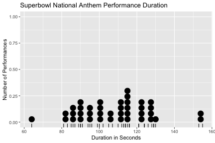<!-- --> ] <style> .panel1-fig_2_2-auto { color: black; width: 38.6060606060606%; hight: 32%; float: left; padding-left: 1%; font-size: 80% } .panel2-fig_2_2-auto { color: black; width: 59.3939393939394%; hight: 32%; float: left; padding-left: 1%; font-size: 80% } .panel3-fig_2_2-auto { color: black; width: NA%; hight: 33%; float: left; padding-left: 1%; font-size: 80% } </style> --- class: center, middle, inverse # Figure 2.3-6 --- count: false .panel1-fig2_3_6-auto[ ```r *prelim_NationalAnthemTimes ``` ] .panel2-fig2_3_6-auto[ ``` # A tibble: 40 × 4 year genre sex time <dbl> <chr> <chr> <dbl> 1 2019 R&B/Soul female 121 2 2018 Pop female 113 3 2017 Country male 124 4 2016 Pop female 129 5 2015 Pop female 124 6 2014 Other female 114 7 2013 Pop female 155 8 2012 Pop female 94 9 2011 Pop female 114 10 2010 Country female 107 11 2009 R&B/Soul female 130 12 2008 Pop female 114 13 2007 Pop male 90 14 2006 R&B/Soul mixed 128 15 2005 Other mixed 112 16 2004 Pop female 129 17 2003 Country female 96 18 2002 Pop female 116 19 2001 Pop male 110 20 2000 Country female 121 21 1999 Pop female 115 22 1998 Pop female 87 23 1997 R&B/Soul male 113 24 1996 Pop female 95 25 1995 Other female 100 26 1994 R&B/Soul female 153 27 1993 Country male 105 28 1992 Pop male 126 29 1991 Pop female 116 30 1990 R&B/Soul male 90 31 1989 Pop male 85 32 1988 Other male 91 33 1987 Pop male 64 34 1986 Other male 83 35 1985 Other mixed 81 36 1984 Pop male 100 37 1983 Other female 102 38 1982 R&B/Soul female 99 39 1981 Pop female 86 40 1980 Pop female 89 ``` ] --- count: false .panel1-fig2_3_6-auto[ ```r prelim_NationalAnthemTimes %>% * names() ``` ] .panel2-fig2_3_6-auto[ ``` [1] "year" "genre" "sex" "time" ``` ] --- count: false .panel1-fig2_3_6-auto[ ```r prelim_NationalAnthemTimes %>% names() *prelim_NationalAnthemTimes ``` ] .panel2-fig2_3_6-auto[ ``` [1] "year" "genre" "sex" "time" ``` ``` # A tibble: 40 × 4 year genre sex time <dbl> <chr> <chr> <dbl> 1 2019 R&B/Soul female 121 2 2018 Pop female 113 3 2017 Country male 124 4 2016 Pop female 129 5 2015 Pop female 124 6 2014 Other female 114 7 2013 Pop female 155 8 2012 Pop female 94 9 2011 Pop female 114 10 2010 Country female 107 11 2009 R&B/Soul female 130 12 2008 Pop female 114 13 2007 Pop male 90 14 2006 R&B/Soul mixed 128 15 2005 Other mixed 112 16 2004 Pop female 129 17 2003 Country female 96 18 2002 Pop female 116 19 2001 Pop male 110 20 2000 Country female 121 21 1999 Pop female 115 22 1998 Pop female 87 23 1997 R&B/Soul male 113 24 1996 Pop female 95 25 1995 Other female 100 26 1994 R&B/Soul female 153 27 1993 Country male 105 28 1992 Pop male 126 29 1991 Pop female 116 30 1990 R&B/Soul male 90 31 1989 Pop male 85 32 1988 Other male 91 33 1987 Pop male 64 34 1986 Other male 83 35 1985 Other mixed 81 36 1984 Pop male 100 37 1983 Other female 102 38 1982 R&B/Soul female 99 39 1981 Pop female 86 40 1980 Pop female 89 ``` ] --- count: false .panel1-fig2_3_6-auto[ ```r prelim_NationalAnthemTimes %>% names() prelim_NationalAnthemTimes %>% * ggplot() ``` ] .panel2-fig2_3_6-auto[ ``` [1] "year" "genre" "sex" "time" ``` <!-- --> ] --- count: false .panel1-fig2_3_6-auto[ ```r prelim_NationalAnthemTimes %>% names() prelim_NationalAnthemTimes %>% ggplot() + * aes(x = time) ``` ] .panel2-fig2_3_6-auto[ ``` [1] "year" "genre" "sex" "time" ``` <!-- --> ] --- count: false .panel1-fig2_3_6-auto[ ```r prelim_NationalAnthemTimes %>% names() prelim_NationalAnthemTimes %>% ggplot() + aes(x = time) + * geom_rug() ``` ] .panel2-fig2_3_6-auto[ ``` [1] "year" "genre" "sex" "time" ``` <!-- --> ] --- count: false .panel1-fig2_3_6-auto[ ```r prelim_NationalAnthemTimes %>% names() prelim_NationalAnthemTimes %>% ggplot() + aes(x = time) + geom_rug() + * geom_histogram() ``` ] .panel2-fig2_3_6-auto[ ``` [1] "year" "genre" "sex" "time" ``` <!-- --> ] --- count: false .panel1-fig2_3_6-auto[ ```r prelim_NationalAnthemTimes %>% names() prelim_NationalAnthemTimes %>% ggplot() + aes(x = time) + geom_rug() + geom_histogram() + * ggxmean::geom_x_mean() ``` ] .panel2-fig2_3_6-auto[ ``` [1] "year" "genre" "sex" "time" ``` <!-- --> ] --- count: false .panel1-fig2_3_6-auto[ ```r prelim_NationalAnthemTimes %>% names() prelim_NationalAnthemTimes %>% ggplot() + aes(x = time) + geom_rug() + geom_histogram() + ggxmean::geom_x_mean() + * ggxmean::geom_x_mean_label() ``` ] .panel2-fig2_3_6-auto[ ``` [1] "year" "genre" "sex" "time" ``` <!-- --> ] --- count: false .panel1-fig2_3_6-auto[ ```r prelim_NationalAnthemTimes %>% names() prelim_NationalAnthemTimes %>% ggplot() + aes(x = time) + geom_rug() + geom_histogram() + ggxmean::geom_x_mean() + ggxmean::geom_x_mean_label() + * ggxmean:::geom_x1sd(lty = "dashed") ``` ] .panel2-fig2_3_6-auto[ ``` [1] "year" "genre" "sex" "time" ``` <!-- --> ] --- count: false .panel1-fig2_3_6-auto[ ```r prelim_NationalAnthemTimes %>% names() prelim_NationalAnthemTimes %>% ggplot() + aes(x = time) + geom_rug() + geom_histogram() + ggxmean::geom_x_mean() + ggxmean::geom_x_mean_label() + ggxmean:::geom_x1sd(lty = "dashed") + * facet_wrap(facets = vars(sex), ncol = 1) ``` ] .panel2-fig2_3_6-auto[ ``` [1] "year" "genre" "sex" "time" ``` <!-- --> ] --- count: false .panel1-fig2_3_6-auto[ ```r prelim_NationalAnthemTimes %>% names() prelim_NationalAnthemTimes %>% ggplot() + aes(x = time) + geom_rug() + geom_histogram() + ggxmean::geom_x_mean() + ggxmean::geom_x_mean_label() + ggxmean:::geom_x1sd(lty = "dashed") + facet_wrap(facets = vars(sex), ncol = 1) + * facet_wrap(facets = vars(genre), ncol = 1) ``` ] .panel2-fig2_3_6-auto[ ``` [1] "year" "genre" "sex" "time" ``` <!-- --> ] --- count: false .panel1-fig2_3_6-auto[ ```r prelim_NationalAnthemTimes %>% names() prelim_NationalAnthemTimes %>% ggplot() + aes(x = time) + geom_rug() + geom_histogram() + ggxmean::geom_x_mean() + ggxmean::geom_x_mean_label() + ggxmean:::geom_x1sd(lty = "dashed") + facet_wrap(facets = vars(sex), ncol = 1) + facet_wrap(facets = vars(genre), ncol = 1) + * facet_grid(rows = vars(sex), cols = vars(genre)) ``` ] .panel2-fig2_3_6-auto[ ``` [1] "year" "genre" "sex" "time" ``` <!-- --> ] --- count: false .panel1-fig2_3_6-auto[ ```r prelim_NationalAnthemTimes %>% names() prelim_NationalAnthemTimes %>% ggplot() + aes(x = time) + geom_rug() + geom_histogram() + ggxmean::geom_x_mean() + ggxmean::geom_x_mean_label() + ggxmean:::geom_x1sd(lty = "dashed") + facet_wrap(facets = vars(sex), ncol = 1) + facet_wrap(facets = vars(genre), ncol = 1) + facet_grid(rows = vars(sex), cols = vars(genre)) + * aes(color = sex) ``` ] .panel2-fig2_3_6-auto[ ``` [1] "year" "genre" "sex" "time" ``` <!-- --> ] <style> .panel1-fig2_3_6-auto { color: black; width: 38.6060606060606%; hight: 32%; float: left; padding-left: 1%; font-size: 80% } .panel2-fig2_3_6-auto { color: black; width: 59.3939393939394%; hight: 32%; float: left; padding-left: 1%; font-size: 80% } .panel3-fig2_3_6-auto { color: black; width: NA%; hight: 33%; float: left; padding-left: 1%; font-size: 80% } </style> --- # 'The best solution to visual dispay of multivariate data is using small multiples' - Eduard Tufte paraphrase -- ### Small multiple: One method Tufte encourages to allow quick visual comparison of multiple series is the small multiple, a chart with many series shown on a single pair of axes that can often be easier to read when displayed as several separate pairs of axes placed next to each other. He suggests this is particularly helpful when the series are measured on quite different vertical (y-axis) scales, but over the same range on the horizontal x-axis (usually time) - wikipedia --- class: center, middle, inverse # Figure 2.8 --- count: false .panel1-fig2_8-auto[ ```r *prelim_NationalAnthemTimes ``` ] .panel2-fig2_8-auto[ ``` # A tibble: 40 × 4 year genre sex time <dbl> <chr> <chr> <dbl> 1 2019 R&B/Soul female 121 2 2018 Pop female 113 3 2017 Country male 124 4 2016 Pop female 129 5 2015 Pop female 124 6 2014 Other female 114 7 2013 Pop female 155 8 2012 Pop female 94 9 2011 Pop female 114 10 2010 Country female 107 11 2009 R&B/Soul female 130 12 2008 Pop female 114 13 2007 Pop male 90 14 2006 R&B/Soul mixed 128 15 2005 Other mixed 112 16 2004 Pop female 129 17 2003 Country female 96 18 2002 Pop female 116 19 2001 Pop male 110 20 2000 Country female 121 21 1999 Pop female 115 22 1998 Pop female 87 23 1997 R&B/Soul male 113 24 1996 Pop female 95 25 1995 Other female 100 26 1994 R&B/Soul female 153 27 1993 Country male 105 28 1992 Pop male 126 29 1991 Pop female 116 30 1990 R&B/Soul male 90 31 1989 Pop male 85 32 1988 Other male 91 33 1987 Pop male 64 34 1986 Other male 83 35 1985 Other mixed 81 36 1984 Pop male 100 37 1983 Other female 102 38 1982 R&B/Soul female 99 39 1981 Pop female 86 40 1980 Pop female 89 ``` ] --- count: false .panel1-fig2_8-auto[ ```r prelim_NationalAnthemTimes %>% * names() ``` ] .panel2-fig2_8-auto[ ``` [1] "year" "genre" "sex" "time" ``` ] --- count: false .panel1-fig2_8-auto[ ```r prelim_NationalAnthemTimes %>% names() *prelim_NationalAnthemTimes ``` ] .panel2-fig2_8-auto[ ``` [1] "year" "genre" "sex" "time" ``` ``` # A tibble: 40 × 4 year genre sex time <dbl> <chr> <chr> <dbl> 1 2019 R&B/Soul female 121 2 2018 Pop female 113 3 2017 Country male 124 4 2016 Pop female 129 5 2015 Pop female 124 6 2014 Other female 114 7 2013 Pop female 155 8 2012 Pop female 94 9 2011 Pop female 114 10 2010 Country female 107 11 2009 R&B/Soul female 130 12 2008 Pop female 114 13 2007 Pop male 90 14 2006 R&B/Soul mixed 128 15 2005 Other mixed 112 16 2004 Pop female 129 17 2003 Country female 96 18 2002 Pop female 116 19 2001 Pop male 110 20 2000 Country female 121 21 1999 Pop female 115 22 1998 Pop female 87 23 1997 R&B/Soul male 113 24 1996 Pop female 95 25 1995 Other female 100 26 1994 R&B/Soul female 153 27 1993 Country male 105 28 1992 Pop male 126 29 1991 Pop female 116 30 1990 R&B/Soul male 90 31 1989 Pop male 85 32 1988 Other male 91 33 1987 Pop male 64 34 1986 Other male 83 35 1985 Other mixed 81 36 1984 Pop male 100 37 1983 Other female 102 38 1982 R&B/Soul female 99 39 1981 Pop female 86 40 1980 Pop female 89 ``` ] --- count: false .panel1-fig2_8-auto[ ```r prelim_NationalAnthemTimes %>% names() prelim_NationalAnthemTimes %>% * ggplot() ``` ] .panel2-fig2_8-auto[ ``` [1] "year" "genre" "sex" "time" ``` <!-- --> ] --- count: false .panel1-fig2_8-auto[ ```r prelim_NationalAnthemTimes %>% names() prelim_NationalAnthemTimes %>% ggplot() + * aes(x = year) ``` ] .panel2-fig2_8-auto[ ``` [1] "year" "genre" "sex" "time" ``` <!-- --> ] --- count: false .panel1-fig2_8-auto[ ```r prelim_NationalAnthemTimes %>% names() prelim_NationalAnthemTimes %>% ggplot() + aes(x = year) + * aes(y = time) ``` ] .panel2-fig2_8-auto[ ``` [1] "year" "genre" "sex" "time" ``` <!-- --> ] --- count: false .panel1-fig2_8-auto[ ```r prelim_NationalAnthemTimes %>% names() prelim_NationalAnthemTimes %>% ggplot() + aes(x = year) + aes(y = time) + * geom_rug() ``` ] .panel2-fig2_8-auto[ ``` [1] "year" "genre" "sex" "time" ``` <!-- --> ] --- count: false .panel1-fig2_8-auto[ ```r prelim_NationalAnthemTimes %>% names() prelim_NationalAnthemTimes %>% ggplot() + aes(x = year) + aes(y = time) + geom_rug() + * geom_point() ``` ] .panel2-fig2_8-auto[ ``` [1] "year" "genre" "sex" "time" ``` <!-- --> ] --- count: false .panel1-fig2_8-auto[ ```r prelim_NationalAnthemTimes %>% names() prelim_NationalAnthemTimes %>% ggplot() + aes(x = year) + aes(y = time) + geom_rug() + geom_point() + * aes(color = sex) ``` ] .panel2-fig2_8-auto[ ``` [1] "year" "genre" "sex" "time" ``` 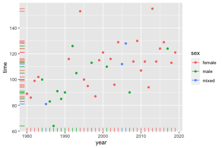<!-- --> ] --- count: false .panel1-fig2_8-auto[ ```r prelim_NationalAnthemTimes %>% names() prelim_NationalAnthemTimes %>% ggplot() + aes(x = year) + aes(y = time) + geom_rug() + geom_point() + aes(color = sex) + * aes(shape = sex) ``` ] .panel2-fig2_8-auto[ ``` [1] "year" "genre" "sex" "time" ``` 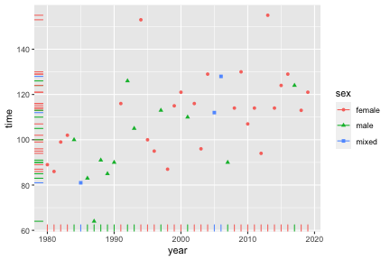<!-- --> ] --- count: false .panel1-fig2_8-auto[ ```r prelim_NationalAnthemTimes %>% names() prelim_NationalAnthemTimes %>% ggplot() + aes(x = year) + aes(y = time) + geom_rug() + geom_point() + aes(color = sex) + aes(shape = sex) + * facet_wrap(facets = vars(sex), ncol = 1) ``` ] .panel2-fig2_8-auto[ ``` [1] "year" "genre" "sex" "time" ``` 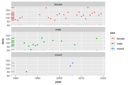<!-- --> ] --- count: false .panel1-fig2_8-auto[ ```r prelim_NationalAnthemTimes %>% names() prelim_NationalAnthemTimes %>% ggplot() + aes(x = year) + aes(y = time) + geom_rug() + geom_point() + aes(color = sex) + aes(shape = sex) + facet_wrap(facets = vars(sex), ncol = 1) + * geom_smooth() # just for fun ``` ] .panel2-fig2_8-auto[ ``` [1] "year" "genre" "sex" "time" ``` 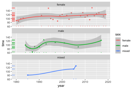<!-- --> ] <style> .panel1-fig2_8-auto { color: black; width: 38.6060606060606%; hight: 32%; float: left; padding-left: 1%; font-size: 80% } .panel2-fig2_8-auto { color: black; width: 59.3939393939394%; hight: 32%; float: left; padding-left: 1%; font-size: 80% } .panel3-fig2_8-auto { color: black; width: NA%; hight: 33%; float: left; padding-left: 1%; font-size: 80% } </style> --- # Fluid plotting/storytelling w/ ggplot2 -- Hadley Wickham, ggplot2 author on it's motivation: > ### And, you know, I'd get a dataset. And, *in my head I could very clearly kind of picture*, I want to put this on the x-axis. Let's put this on the y-axis, draw a line, put some points here, break it up by this variable. -- > ### And then, like, getting that vision out of my head, and into reality, it's just really, really hard. Just, like, felt harder than it should be. Like, there's a lot of custom programming involved, --- > ### where I just felt, like, to me, I just wanted to say, like, you know, *this is what I'm thinking, this is how I'm picturing this plot. Like you're the computer 'Go and do it'.* -- > ### ... and I'd also been reading about the Grammar of Graphics by Leland Wilkinson, I got to meet him a couple of times and ... I was, like, this book has been, like, written for me. https://www.trifacta.com/podcast/tidy-data-with-hadley-wickham/ --- # Summarizing: -- Promise of ggplot2? -- ## Getting the plot form you picture in your head ... -- ## ... into reality... -- ## ... by describing it. --- class: inverse, center, middle # Intentional data communication ... -- # mirrors intentional step-by-step data exploration! -- # give decisions full voice. Move slowly and with intention. +1 for + aes() Dr. Reynolds rant --- # ggplot2 is called a 'declarative' graphing system. -- # It lets you *'speak your plot into existence'*. (Thomas Lin Pederson?) --- # Other examples: # https://evamaerey.github.io/mytidytuesday/2022-07-22-ma206data-demo/ma206data_package_demo.html