Using ggplot2 has been described as writing ‘graphical poems’. But we may feel at a loss for ‘words’ when functions we’d like to have don’t exist. The ggplot2 extension system allows us to build new ‘vocabulary’ for fluent expression.
An exciting extension mechanism is that of inheriting from existing, more primitive geom behavior after performing some calculation.
To get your feet wet in this world and give you a taste of patterns for geom extension, we provide three basic examples of the geoms_ that use primitive geoms (GeomPoint, GeomText, GeomSegment, etc) along with a practice exercise. With such geom_ (or stat_) functions, calculation is done under the hood by the ggplot2 system. You may only be familiar with the user-facing geom_point(), geom_text(), geom_segment() layer functions that use these more primitive objects under the hood, and that’s okay - this should give you enough intuition for using primitives.
With these geom_ functions, you can write new graphical poems with concise new ‘words’ you’ve designed yourself!
This tutorial is intended for individuals who already have a solid working knowledge of the syntax of ggplot2 but may like to build a richer layer vocabulary for themselves.
Overview
Our recipes take the form:
Step 0. Get the job done with ‘base’ ggplot2. It’s a good idea to clarify what needs to happen without getting into the extension architecture
Step 1.a Write a computation function. Wrap the necessary computation into a function that your target geom_*() function will perform. We focus on ‘compute_group’ computation only in this tutorial.
Step 1.b Test using prepped data
Step 2.a Define a Stat ggproto objects allow your extension to work together with base ggplot2 functions! You’ll use the computation function from step 1 to help define it.
Step 2.b Test Stat
Step 3.a Write user-facing function! You’re ready to write your function. You will incorporate the ggproto from Step 2 and also define which more primitive geom (point, text, segment etc) you want other behaviors to inherit from.
Step 3.b Test. Enjoy! Take your new geom for a spin! Check out group-wise computation behavior!
Below, you’ll see a completely worked example (example recipes A, B and C) and then a invitation to build a related target geom_*() (Tasks A, B, and C).
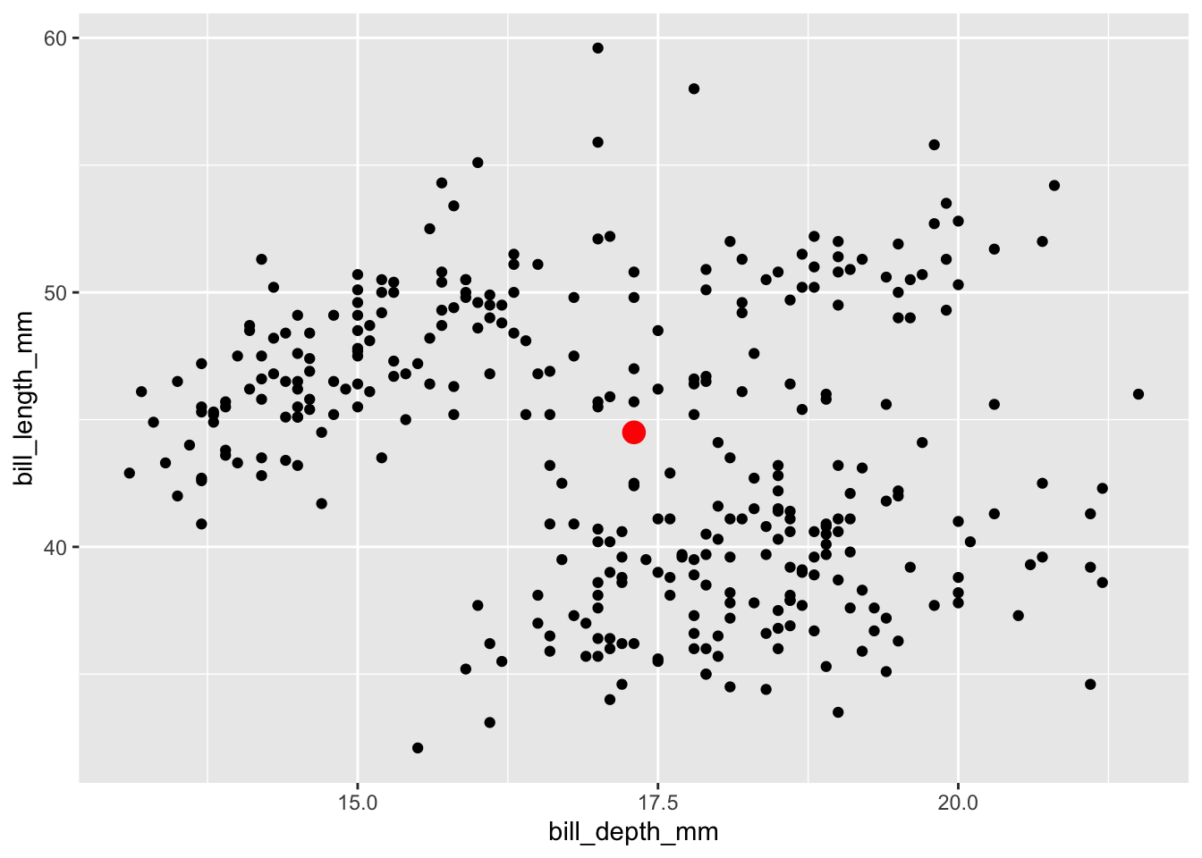
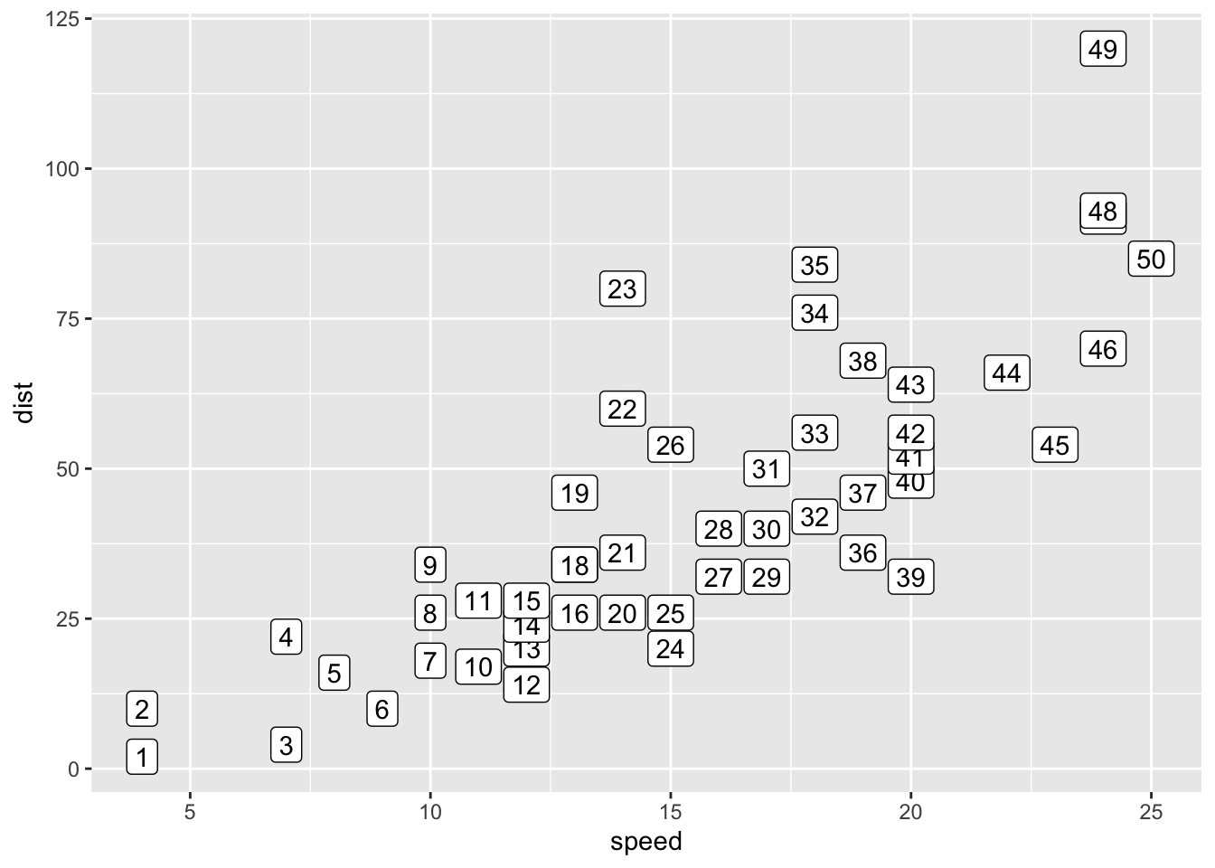
define computation that ggplot2 should do for you, before plotting
here it’s computing a variable with labels for each observation
test that functionality Step 1.b
# Step 1.acompute_group_xy_medians <-function(data, scales){ # scales is used internally in ggplot2 data %>%summarize(x =median(x),y =median(y))}
Step 1b. Test compute
penguins |>select(x = bill_depth_mm, # ggplot2 will work with 'aes' column namesy = bill_length_mm) |># therefore select is required to used the compute functioncompute_group_xy_medians()
# A tibble: 1 × 2
      x     y
  <dbl> <dbl>
1  17.3  44.5
Step 2: define new Stat
Things to notice
what’s the naming convention for the proto object?
Step 2b. Test. Use the stat with long-form, layer() function.
Step 3a: define geom_* function
Things to notice
Where does our work up to this point enter in?
What more primitive geom will we inherit behavior from?
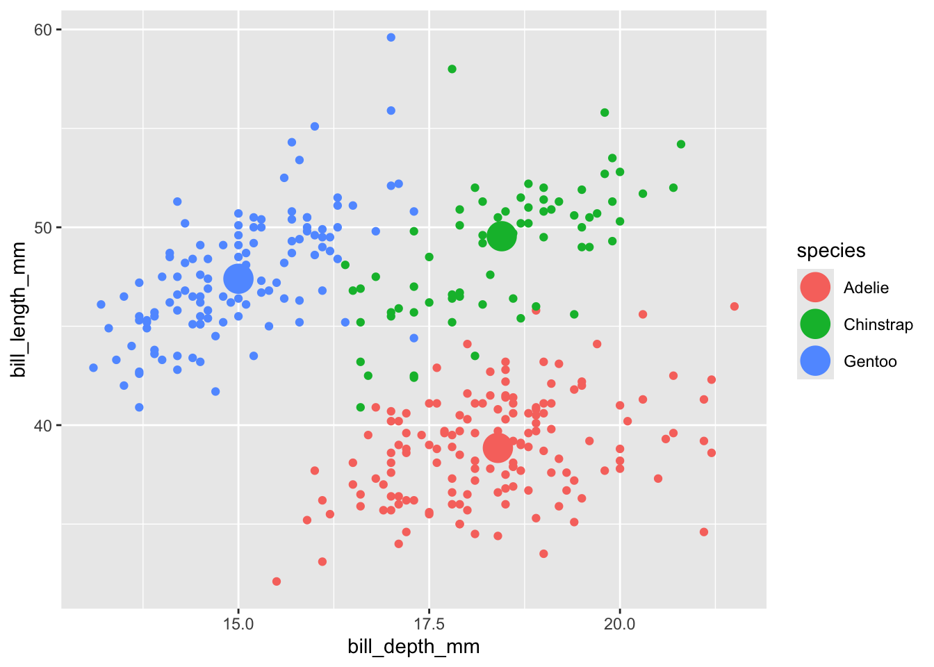
geom_point_xy_medians <-function(mapping =NULL, # global aesthetics will be used if NULLdata =NULL, # global data will be used if NULLposition ="identity", na.rm =FALSE, show.legend =NA,inherit.aes =TRUE, ... # many other arguments can be used specific to # the Geom thats used in layer and to computation definition ) { ggplot2::layer(stat = StatXymedians, geom = ggplot2::GeomPoint, data = data, mapping = mapping,position = position, show.legend = show.legend, inherit.aes = inherit.aes,params =list(na.rm = na.rm, ...) )}
penguins |>ggplot()+aes(x = bill_depth_mm, y = bill_length_mm, color = species)+geom_point()+geom_point_xy_medians(size =7)
Task #A: create the function geom_point_xy_means()
Using recipe #1 as a reference, try to create the function geom_point_xy_means()
# step 0: use base ggplot2

# step 1: write your compute_group function - don't forget scales argument!

# step 2: write ggproto with compute_group as an input

# step 3: write your geom_*() function with ggproto as an input

# step 4: enjoy!
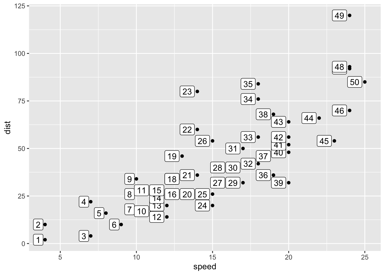
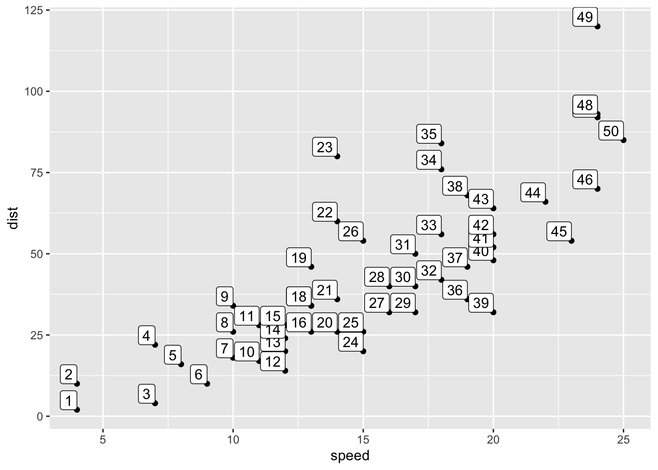
# you won't use the scales argument, but ggplot will latercompute_group_row_number <-function(data, scales){ data |># add an additional column called label# the geom we inherit from requires the label aestheticmutate(label =1:n())}
Step 1b test the computation function
cars |># input must have required aesthetic inputs as columnsselect(x = speed, y = dist) |>compute_group_row_number() |>head()
cars |>ggplot() +aes(x = speed, y = dist) +geom_point() +geom_label_row_number(hjust =1,vjust =0) # function in action
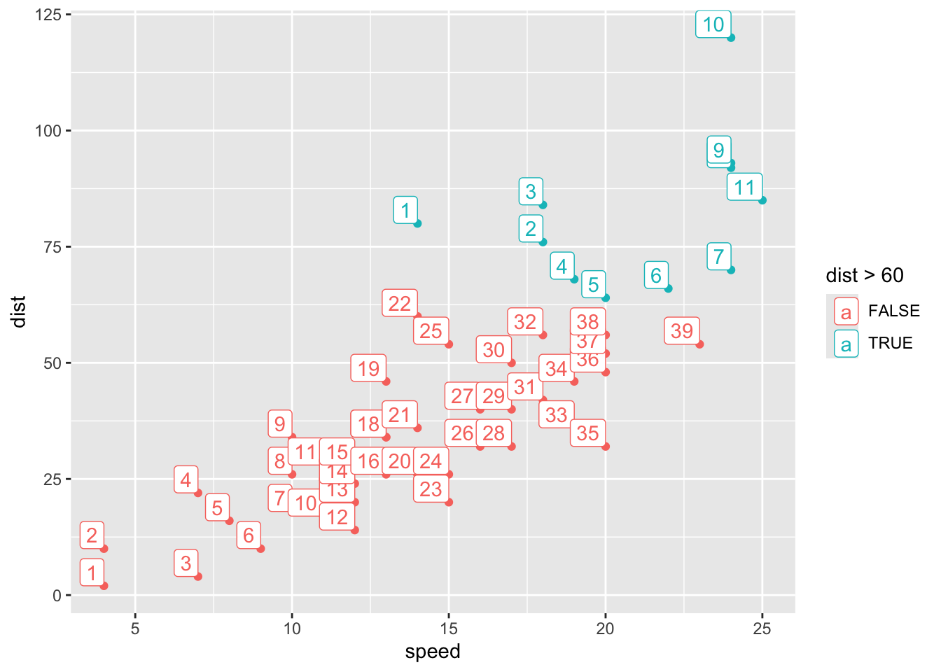
And check out conditionality!
last_plot() +aes(color = dist >60) # Computation is within group
Task #B: create geom_text_coordinates()
Using recipe #2 as a reference, can you create the function geom_text_coordinates().
–
geom should label point with its coordinates ‘(x, y)’
geom should have behavior of geom_text (not geom_label)
Hint:
paste0("(", 1, ", ", 3.5, ")")
[1] "(1, 3.5)"
# step 0: use base ggplot2

# step 1: write your compute_group function (and test)

# step 2: write ggproto with compute_group as an input

# step 3: write your geom_*() function with ggproto as an input

# step 4: enjoy!
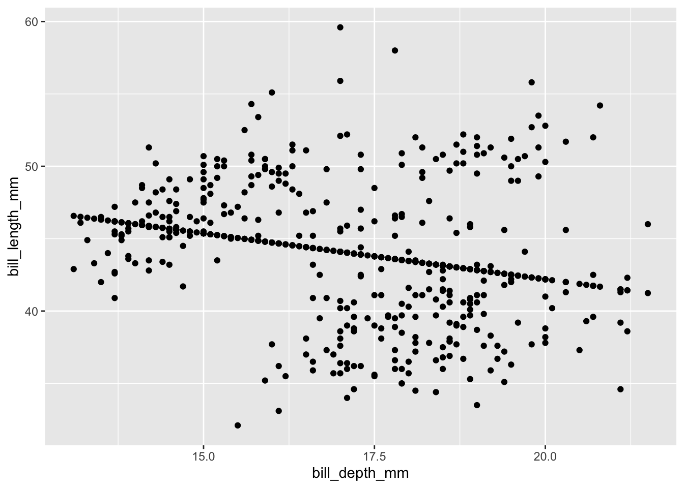
Example recipe #C: geom_point_lm_fitted()
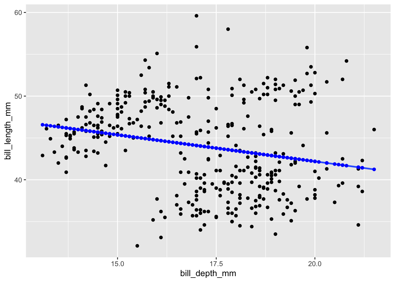
Step 0: use base ggplot2 to get the job done
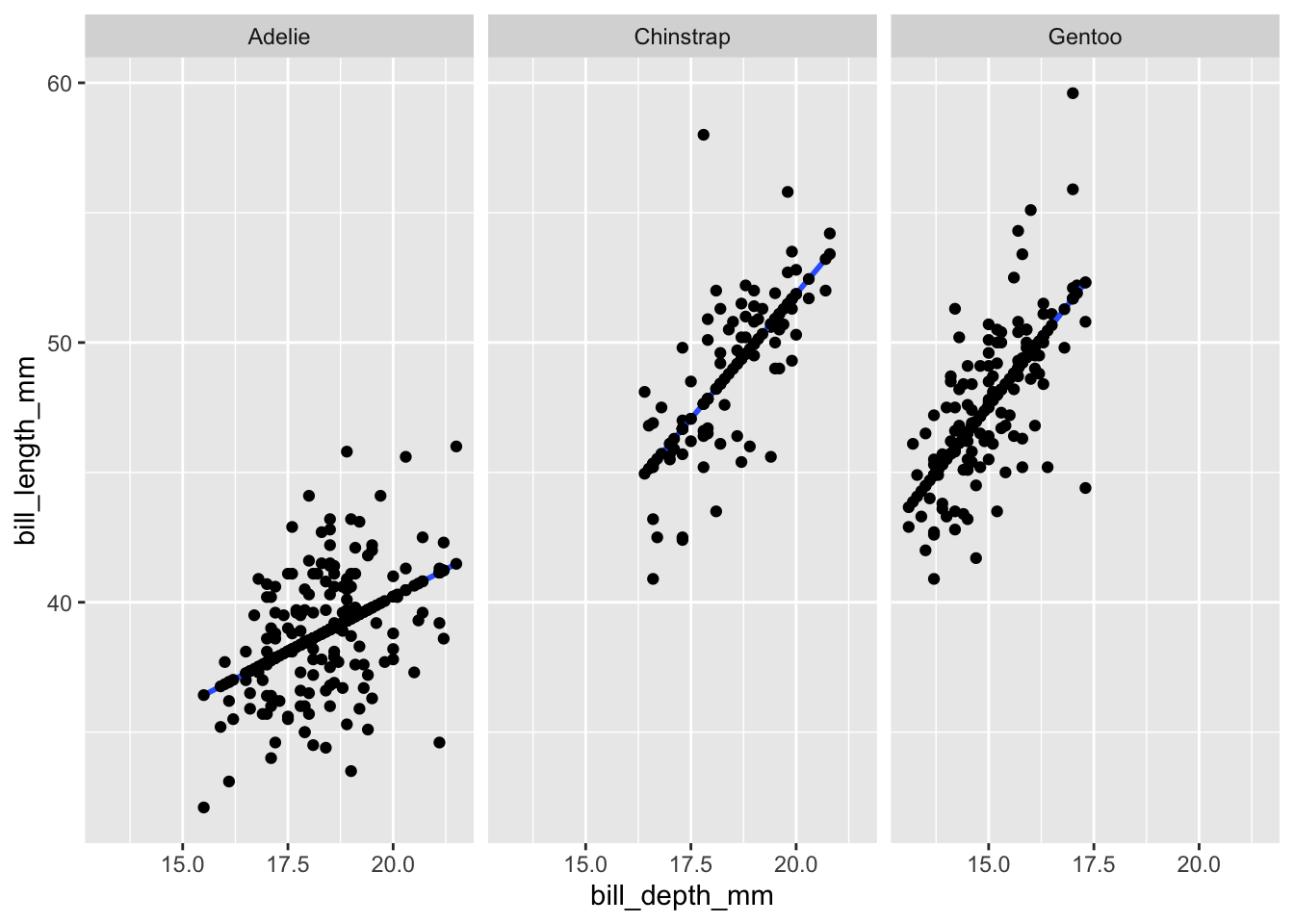
model <-lm(formula = bill_length_mm ~ bill_depth_mm, data = penguins) penguins_w_fitted <- penguins |>mutate(fitted = model$fitted.values)penguins |>ggplot() +aes(x = bill_depth_mm, y = bill_length_mm) +geom_point() +geom_smooth(method ="lm", se = F) +geom_point(data = penguins_w_fitted,aes(y = fitted),color ="blue")
Step 1a: write compute function
compute_group_lm_fitted <-function(data, scales){ model<-lm(formula= y ~ x, data = data) data |>mutate(y = model$fitted.values)}
Step 1b. test out the function
penguins |># select to explicitly state the x and y inputsselect(x = bill_depth_mm, y = bill_length_mm)|>compute_group_lm_fitted()