1. Snappy Title: Predictive Power and the Palmer Penguins

class: center, middle, inverse, title-slide

# 1. Snappy Title: Predictive Power and the Palmer Penguins
## 2. Descriptive title: Does bill length predict bill depth?
### 3. Authors: Dr. Reynolds

---

## 4. A compelling visual that has to do with your question:

![](https://allisonhorst.github.io/palmerpenguins/reference/figures/culmen_depth.png)

---

![](https://allisonhorst.github.io/palmerpenguins/reference/figures/lter_penguins.png)

---

### 5. Background summary paragraph and data origins:

### This study seeks to explore the relationship between features of the 'Palmer Penguins'.  
--
There are 344 penguins whose measurements we have.  
--
We will look at the relationships between the following four variables using linear regression modeling.  
--
The data was originally published in 'Gorman KB, Williams TD, Fraser WR (2014).
--
Ecological sexual dimorphism and environmental variability within a community of Antarctic penguins';
--
and we are using the cleaned data available in the Palmer Penguin R package (Horst AM, Hill AP, Gorman KB (2020)).

---

## 6. Snapshot of the variables of interest...

```r
palmerpenguins::penguins %>%
  select(bill_length_mm,
         bill_depth_mm,
         species,
         sex)
```

```
# A tibble: 344 × 4
   bill_length_mm bill_depth_mm species sex   
            <dbl>         <dbl> <fct>   <fct> 
 1           39.1          18.7 Adelie  male  
 2           39.5          17.4 Adelie  female
 3           40.3          18   Adelie  female
 4           NA            NA   Adelie  <NA>  
 5           36.7          19.3 Adelie  female
 6           39.3          20.6 Adelie  male  
 7           38.9          17.8 Adelie  female
 8           39.2          19.6 Adelie  male  
 9           34.1          18.1 Adelie  <NA>  
10           42            20.2 Adelie  <NA>  
# … with 334 more rows
```

---

## 7. What other research finds (2 sources):

### a. Other researchers (Gorman et al 2014) found that there was a relationship between flipper length and body mass within species. Given this finding, it is plausible that relationships between other features exist.

### b. Furthermore, it is well known (Fracis 2002; Miller 2010) that animal sex can impact the size of animal features.

---

## 8. Univariate distributions (1 for each of 4 variables)

### Distributions in dataset for categorical variables:

```r
palmerpenguins::penguins %>%
  ggplot() +
  aes(x = species) +
  geom_bar()
```

![](penguins_presentation_files/figure-html/unnamed-chunk-3-1.png)

---

### Distributions in dataset for categorical variables:

```r
palmerpenguins::penguins %>%
  ggplot() +
  aes(x = sex) +
  geom_bar()
```

![](penguins_presentation_files/figure-html/unnamed-chunk-4-1.png)

---

### Distributions in dataset for continuous variables:

```r
palmerpenguins::penguins %>%
  ggplot() +
  aes(x = bill_length_mm) +
  geom_histogram()
```

![](penguins_presentation_files/figure-html/unnamed-chunk-5-1.png)

---

### Distributions in dataset for continuous variables:

```r
palmerpenguins::penguins %>%
  ggplot() +
  aes(x = bill_depth_mm) +
  geom_histogram()
```

![](penguins_presentation_files/figure-html/unnamed-chunk-6-1.png)

---

#### 9. Bivariate relationship.  Just show relationship of two *variables of interest.*

```r
palmerpenguins::penguins %>%
  ggplot() +
  aes(y = bill_depth_mm,
      x = bill_length_mm) +
  geom_point()
```

![](penguins_presentation_files/figure-html/unnamed-chunk-7-1.png)

---

#### 10. Multivariate relationship

Try to visualize all variables of interest using various visual channels (x and y position, color, shape, etc)

```r
palmerpenguins::penguins %>%
  ggplot() +
  aes(y = bill_depth_mm,
      x = bill_length_mm,
      color = species,
      shape = sex
      ) +
  geom_point()
```

![](penguins_presentation_files/figure-html/unnamed-chunk-8-1.png)

---

#### 11.a Estimate model...

```r
palmerpenguins::penguins %>%
  lm(bill_depth_mm ~ bill_length_mm + sex + species, data = .) ->
lrmodel

print(lrmodel)
```

```

Call:
lm(formula = bill_depth_mm ~ bill_length_mm + sex + species, 
    data = .)

Coefficients:
     (Intercept)    bill_length_mm           sexmale  speciesChinstrap  
        15.07161           0.06824           1.25285          -0.60971  
   speciesGentoo  
        -3.96308  
```

---

#### 11.b Modeling

Write out model specification (use betas):

`$$\hat{y} = \beta_0 + \beta_1*bill_length_mm + \beta_2*male + \beta_3*Chinstrap + \beta_1*Gentoo$$`
---

#### 11.c Rewrite model with numerical values:

`$$bill\_depth = 15.0716  + 0.0682*bill\_length\_mm + 1.2528*male + -0.6097*Chinstrap + -3.9631*Gentoo$$`

---

#### 11.d Discussion of model relationships

### There is a positive association between bill depth and bill length when controlling for sex and species.  
--
For every 1 mm increase in bill depth, we expect a .068 mm increase in bill depth.  
--
For male birds vs. the baseline category (female) birds, holding everything else equal, we expect the bill length to be 1.25 mm longer.
--
Gentoo's bill depth are expected to be shortest among these animals, w/ an expected decrease of 3.96 mm greater length expected relative to Adelie Penguin's (baseline category) of same characteristics otherwise (i.e. same bill depth, same sex).  Chinstraps are also expected to have shorter bill depths by .609 compared with baseline category (Adelie).

---

#### 12.a Full model summary

```r
summary(lrmodel)
```

```

Call:
lm(formula = bill_depth_mm ~ bill_length_mm + sex + species, 
    data = .)

Residuals:
     Min       1Q   Median       3Q      Max 
-2.10170 -0.54971 -0.07144  0.49233  2.92621

Coefficients:
                 Estimate Std. Error t value Pr(>|t|)    
(Intercept)      15.07161    0.72264  20.856  < 2e-16 ***
bill_length_mm    0.06824    0.01942   3.514 0.000504 ***
sexmale           1.25285    0.11489  10.904  < 2e-16 ***
speciesChinstrap -0.60971    0.22855  -2.668 0.008015 ** 
speciesGentoo    -3.96308    0.19686 -20.132  < 2e-16 ***
---
Signif. codes:  0 '***' 0.001 '**' 0.01 '*' 0.05 '.' 0.1 ' ' 1

Residual standard error: 0.8188 on 328 degrees of freedom
  (11 observations deleted due to missingness)
Multiple R-squared:  0.8292,	Adjusted R-squared:  0.8271 
F-statistic: 398.1 on 4 and 328 DF,  p-value: < 2.2e-16
```

---

# 12.b Discussion of variance explained and statistical significance

## Given the model summary output, we see that the R-squared .82; much of the variance for bill length is explained by this model!  
--
Looking at the p-values associated with the modeling coefficients, we see very small p-values in every Beta coefficient .  
--
The coefficients are statistically significant at the alpha = .05 level (they are inconsistent with being the value zero).

---

# 13 Validity conditions

```r
lrmodel %>%
  fortify(lrmodel$model) %>%
  ggplot(aes(x = .fitted,
             y = .resid)) +
  geom_point() +
  geom_hline(yintercept = 0) +
  labs( x = "Predicted Values",
        y = "Residuals",
        title = "Residuals vs. predicted values")
```

![](penguins_presentation_files/figure-html/unnamed-chunk-11-1.png)

13a Linearity and equal variance: residuals don't show signs of non-linearity (aren't above the line then below then above).  However, residuals variance does increase as prediction values increase; a bit of concern for equal variance requirement.

---

### 13b Independance condition

#### seeing some waves here... Hints at a problem

```r
lrmodel%>%
  fortify(lrmodel$model) %>%
  mutate(row = row_number()) %>%
  ggplot(aes(x = row,
             y = .resid))+
  geom_point()+
  geom_hline(yintercept = 0)+
  labs(x = "Order of Occurence",
       y = "Residuals",
       title = "Residuals in Order of Occurence")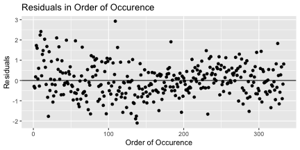
```

![](penguins_presentation_files/figure-html/unnamed-chunk-12-1.png)

---

## 13.c Normality of residuals

```r
lrmodel%>%
  fortify(lrmodel$model)%>%
  ggplot(aes(x = .resid))+
  geom_histogram()+
  labs(x = "Residuals",
       title = "Histogram of residuals")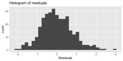
```

![](penguins_presentation_files/figure-html/unnamed-chunk-13-1.png)

### Looks pretty bell shaped. Not worried about this one.

@media print {
  .has-continuation {
    display: block;
  }
}

</style>