count: false .panel1-the_chunk-auto[ ``` r *library(dsbox) ``` ] .panel2-the_chunk-auto[ ] --- count: false .panel1-the_chunk-auto[ ``` r library(dsbox) *dcbikeshare ``` ] .panel2-the_chunk-auto[ ``` # A tibble: 731 × 16 instant dteday season yr mnth holiday weekday workingday weathersit <dbl> <date> <dbl> <dbl> <dbl> <dbl> <dbl> <dbl> <dbl> 1 1 2011-01-01 1 0 1 0 6 0 2 2 2 2011-01-02 1 0 1 0 0 0 2 3 3 2011-01-03 1 0 1 0 1 1 1 4 4 2011-01-04 1 0 1 0 2 1 1 5 5 2011-01-05 1 0 1 0 3 1 1 6 6 2011-01-06 1 0 1 0 4 1 1 7 7 2011-01-07 1 0 1 0 5 1 2 8 8 2011-01-08 1 0 1 0 6 0 2 9 9 2011-01-09 1 0 1 0 0 0 1 10 10 2011-01-10 1 0 1 0 1 1 1 # ℹ 721 more rows # ℹ 7 more variables: temp <dbl>, atemp <dbl>, hum <dbl>, windspeed <dbl>, # casual <dbl>, registered <dbl>, cnt <dbl> ``` ] --- count: false .panel1-the_chunk-auto[ ``` r library(dsbox) dcbikeshare %>% * mutate(atemp_raw = atemp * 50) ``` ] .panel2-the_chunk-auto[ ``` # A tibble: 731 × 17 instant dteday season yr mnth holiday weekday workingday weathersit <dbl> <date> <dbl> <dbl> <dbl> <dbl> <dbl> <dbl> <dbl> 1 1 2011-01-01 1 0 1 0 6 0 2 2 2 2011-01-02 1 0 1 0 0 0 2 3 3 2011-01-03 1 0 1 0 1 1 1 4 4 2011-01-04 1 0 1 0 2 1 1 5 5 2011-01-05 1 0 1 0 3 1 1 6 6 2011-01-06 1 0 1 0 4 1 1 7 7 2011-01-07 1 0 1 0 5 1 2 8 8 2011-01-08 1 0 1 0 6 0 2 9 9 2011-01-09 1 0 1 0 0 0 1 10 10 2011-01-10 1 0 1 0 1 1 1 # ℹ 721 more rows # ℹ 8 more variables: temp <dbl>, atemp <dbl>, hum <dbl>, windspeed <dbl>, # casual <dbl>, registered <dbl>, cnt <dbl>, atemp_raw <dbl> ``` ] --- count: false .panel1-the_chunk-auto[ ``` r library(dsbox) dcbikeshare %>% mutate(atemp_raw = atemp * 50) %>% * ggplot() ``` ] .panel2-the_chunk-auto[ <!-- --> ] --- count: false .panel1-the_chunk-auto[ ``` r library(dsbox) dcbikeshare %>% mutate(atemp_raw = atemp * 50) %>% ggplot() + * aes(x = dteday, y = cnt) ``` ] .panel2-the_chunk-auto[ <!-- --> ] --- count: false .panel1-the_chunk-auto[ ``` r library(dsbox) dcbikeshare %>% mutate(atemp_raw = atemp * 50) %>% ggplot() + aes(x = dteday, y = cnt) + * geom_point() ``` ] .panel2-the_chunk-auto[ 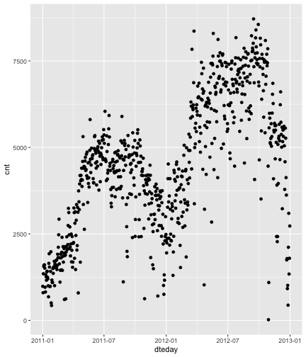<!-- --> ] --- count: false .panel1-the_chunk-auto[ ``` r library(dsbox) dcbikeshare %>% mutate(atemp_raw = atemp * 50) %>% ggplot() + aes(x = dteday, y = cnt) + geom_point() + * labs(title = "Bike rentals in DC, 2011 and 2012", * subtitle = "Warmer temperatures associated with more bike rentals", * x = "Date", * y = "Bike renrals", * color = "Temperature (C)") ``` ] .panel2-the_chunk-auto[ <!-- --> ] --- count: false .panel1-the_chunk-auto[ ``` r library(dsbox) dcbikeshare %>% mutate(atemp_raw = atemp * 50) %>% ggplot() + aes(x = dteday, y = cnt) + geom_point() + labs(title = "Bike rentals in DC, 2011 and 2012", subtitle = "Warmer temperatures associated with more bike rentals", x = "Date", y = "Bike renrals", color = "Temperature (C)") + * theme_minimal() ``` ] .panel2-the_chunk-auto[ 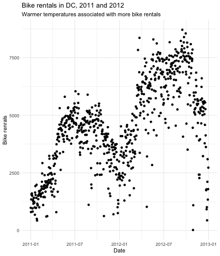<!-- --> ] --- count: false .panel1-the_chunk-auto[ ``` r library(dsbox) dcbikeshare %>% mutate(atemp_raw = atemp * 50) %>% ggplot() + aes(x = dteday, y = cnt) + geom_point() + labs(title = "Bike rentals in DC, 2011 and 2012", subtitle = "Warmer temperatures associated with more bike rentals", x = "Date", y = "Bike renrals", color = "Temperature (C)") + theme_minimal() + * geom_lm(alpha = .2) ``` ] .panel2-the_chunk-auto[ <!-- --> ] --- count: false .panel1-the_chunk-auto[ ``` r library(dsbox) dcbikeshare %>% mutate(atemp_raw = atemp * 50) %>% ggplot() + aes(x = dteday, y = cnt) + geom_point() + labs(title = "Bike rentals in DC, 2011 and 2012", subtitle = "Warmer temperatures associated with more bike rentals", x = "Date", y = "Bike renrals", color = "Temperature (C)") + theme_minimal() + geom_lm(alpha = .2) + * geom_text(stat = StatLmGlance, size = 5) ``` ] .panel2-the_chunk-auto[ <!-- --> ] --- count: false .panel1-the_chunk-auto[ ``` r library(dsbox) dcbikeshare %>% mutate(atemp_raw = atemp * 50) %>% ggplot() + aes(x = dteday, y = cnt) + geom_point() + labs(title = "Bike rentals in DC, 2011 and 2012", subtitle = "Warmer temperatures associated with more bike rentals", x = "Date", y = "Bike renrals", color = "Temperature (C)") + theme_minimal() + geom_lm(alpha = .2) + geom_text(stat = StatLmGlance, size = 5) + * stat_lm(geom = 'segment', alpha = .2) ``` ] .panel2-the_chunk-auto[ 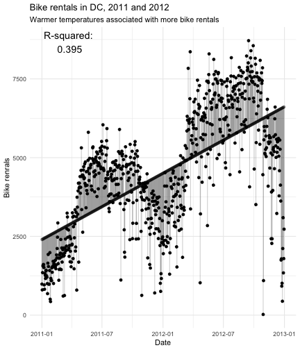<!-- --> ] --- count: false .panel1-the_chunk-auto[ ``` r library(dsbox) dcbikeshare %>% mutate(atemp_raw = atemp * 50) %>% ggplot() + aes(x = dteday, y = cnt) + geom_point() + labs(title = "Bike rentals in DC, 2011 and 2012", subtitle = "Warmer temperatures associated with more bike rentals", x = "Date", y = "Bike renrals", color = "Temperature (C)") + theme_minimal() + geom_lm(alpha = .2) + geom_text(stat = StatLmGlance, size = 5) + stat_lm(geom = 'segment', alpha = .2) + * aes(season = as.factor(season)) ``` ] .panel2-the_chunk-auto[ <!-- --> ] --- count: false .panel1-the_chunk-auto[ ``` r library(dsbox) dcbikeshare %>% mutate(atemp_raw = atemp * 50) %>% ggplot() + aes(x = dteday, y = cnt) + geom_point() + labs(title = "Bike rentals in DC, 2011 and 2012", subtitle = "Warmer temperatures associated with more bike rentals", x = "Date", y = "Bike renrals", color = "Temperature (C)") + theme_minimal() + geom_lm(alpha = .2) + geom_text(stat = StatLmGlance, size = 5) + stat_lm(geom = 'segment', alpha = .2) + aes(season = as.factor(season)) + * aes(holiday = holiday) ``` ] .panel2-the_chunk-auto[ <!-- --> ] --- count: false .panel1-the_chunk-auto[ ``` r library(dsbox) dcbikeshare %>% mutate(atemp_raw = atemp * 50) %>% ggplot() + aes(x = dteday, y = cnt) + geom_point() + labs(title = "Bike rentals in DC, 2011 and 2012", subtitle = "Warmer temperatures associated with more bike rentals", x = "Date", y = "Bike renrals", color = "Temperature (C)") + theme_minimal() + geom_lm(alpha = .2) + geom_text(stat = StatLmGlance, size = 5) + stat_lm(geom = 'segment', alpha = .2) + aes(season = as.factor(season)) + aes(holiday = holiday) + * aes(shape = ind2cat::ind_recode(workingday)) + labs(shape = NULL) ``` ] .panel2-the_chunk-auto[ <!-- --> ] --- count: false .panel1-the_chunk-auto[ ``` r library(dsbox) dcbikeshare %>% mutate(atemp_raw = atemp * 50) %>% ggplot() + aes(x = dteday, y = cnt) + geom_point() + labs(title = "Bike rentals in DC, 2011 and 2012", subtitle = "Warmer temperatures associated with more bike rentals", x = "Date", y = "Bike renrals", color = "Temperature (C)") + theme_minimal() + geom_lm(alpha = .2) + geom_text(stat = StatLmGlance, size = 5) + stat_lm(geom = 'segment', alpha = .2) + aes(season = as.factor(season)) + aes(holiday = holiday) + aes(shape = ind2cat::ind_recode(workingday)) + labs(shape = NULL) + * aes(workingday = workingday) ``` ] .panel2-the_chunk-auto[ <!-- --> ] --- count: false .panel1-the_chunk-auto[ ``` r library(dsbox) dcbikeshare %>% mutate(atemp_raw = atemp * 50) %>% ggplot() + aes(x = dteday, y = cnt) + geom_point() + labs(title = "Bike rentals in DC, 2011 and 2012", subtitle = "Warmer temperatures associated with more bike rentals", x = "Date", y = "Bike renrals", color = "Temperature (C)") + theme_minimal() + geom_lm(alpha = .2) + geom_text(stat = StatLmGlance, size = 5) + stat_lm(geom = 'segment', alpha = .2) + aes(season = as.factor(season)) + aes(holiday = holiday) + aes(shape = ind2cat::ind_recode(workingday)) + labs(shape = NULL) + aes(workingday = workingday) + * aes(color = atemp_raw) + aes(atemp_raw = atemp_raw) ``` ] .panel2-the_chunk-auto[ <!-- --> ] --- count: false .panel1-the_chunk-auto[ ``` r library(dsbox) dcbikeshare %>% mutate(atemp_raw = atemp * 50) %>% ggplot() + aes(x = dteday, y = cnt) + geom_point() + labs(title = "Bike rentals in DC, 2011 and 2012", subtitle = "Warmer temperatures associated with more bike rentals", x = "Date", y = "Bike renrals", color = "Temperature (C)") + theme_minimal() + geom_lm(alpha = .2) + geom_text(stat = StatLmGlance, size = 5) + stat_lm(geom = 'segment', alpha = .2) + aes(season = as.factor(season)) + aes(holiday = holiday) + aes(shape = ind2cat::ind_recode(workingday)) + labs(shape = NULL) + aes(workingday = workingday) + aes(color = atemp_raw) + aes(atemp_raw = atemp_raw) + * aes(dteday = dteday) ``` ] .panel2-the_chunk-auto[ <!-- --> ] --- count: false .panel1-the_chunk-auto[ ``` r library(dsbox) dcbikeshare %>% mutate(atemp_raw = atemp * 50) %>% ggplot() + aes(x = dteday, y = cnt) + geom_point() + labs(title = "Bike rentals in DC, 2011 and 2012", subtitle = "Warmer temperatures associated with more bike rentals", x = "Date", y = "Bike renrals", color = "Temperature (C)") + theme_minimal() + geom_lm(alpha = .2) + geom_text(stat = StatLmGlance, size = 5) + stat_lm(geom = 'segment', alpha = .2) + aes(season = as.factor(season)) + aes(holiday = holiday) + aes(shape = ind2cat::ind_recode(workingday)) + labs(shape = NULL) + aes(workingday = workingday) + aes(color = atemp_raw) + aes(atemp_raw = atemp_raw) + aes(dteday = dteday) + * aes(x = atemp_raw) ``` ] .panel2-the_chunk-auto[ <!-- --> ] --- count: false .panel1-the_chunk-auto[ ``` r library(dsbox) dcbikeshare %>% mutate(atemp_raw = atemp * 50) %>% ggplot() + aes(x = dteday, y = cnt) + geom_point() + labs(title = "Bike rentals in DC, 2011 and 2012", subtitle = "Warmer temperatures associated with more bike rentals", x = "Date", y = "Bike renrals", color = "Temperature (C)") + theme_minimal() + geom_lm(alpha = .2) + geom_text(stat = StatLmGlance, size = 5) + stat_lm(geom = 'segment', alpha = .2) + aes(season = as.factor(season)) + aes(holiday = holiday) + aes(shape = ind2cat::ind_recode(workingday)) + labs(shape = NULL) + aes(workingday = workingday) + aes(color = atemp_raw) + aes(atemp_raw = atemp_raw) + aes(dteday = dteday) + aes(x = atemp_raw) + * aes(weathersit = as.factor(weathersit)) ``` ] .panel2-the_chunk-auto[ 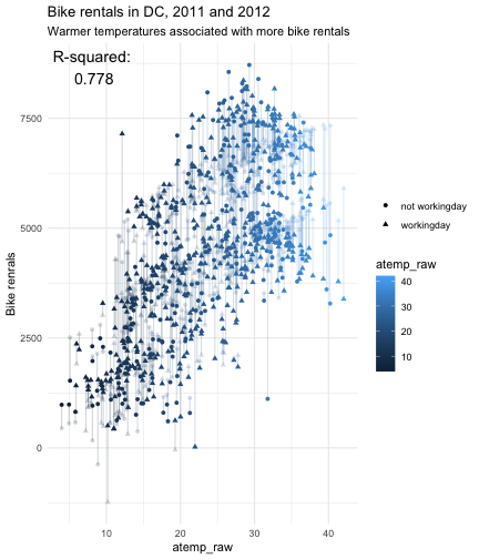<!-- --> ] <style> .panel1-the_chunk-auto { color: black; width: 38.6060606060606%; hight: 32%; float: left; padding-left: 1%; font-size: 80% } .panel2-the_chunk-auto { color: black; width: 59.3939393939394%; hight: 32%; float: left; padding-left: 1%; font-size: 80% } .panel3-the_chunk-auto { color: black; width: NA%; hight: 33%; float: left; padding-left: 1%; font-size: 80% } </style> --- ``` r return_model() ``` ``` Call: lm(formula = formula, data = lmdata) Residuals: Min 1Q Median 3Q Max -3753.2 -390.5 60.6 540.0 3648.6 Coefficients: (3 not defined because of singularities) Estimate Std. Error t value Pr(>|t|) (Intercept) -7.558e+04 2.710e+03 -27.890 < 2e-16 *** weathersit2 -6.523e+02 7.311e+01 -8.921 < 2e-16 *** weathersit3 -2.518e+03 2.073e+02 -12.145 < 2e-16 *** x 1.068e+02 7.287e+00 14.658 < 2e-16 *** dteday 5.042e+00 1.782e-01 28.298 < 2e-16 *** atemp_raw NA NA NA NA colour NA NA NA NA workingday 1.499e+02 7.585e+01 1.977 0.048463 * shapeworkingday NA NA NA NA holiday -6.655e+02 2.107e+02 -3.159 0.001649 ** season2 9.366e+02 1.258e+02 7.443 2.81e-13 *** season3 3.330e+02 1.621e+02 2.054 0.040342 * season4 4.096e+02 1.132e+02 3.619 0.000316 *** --- Signif. codes: 0 '***' 0.001 '**' 0.01 '*' 0.05 '.' 0.1 ' ' 1 Residual standard error: 919.2 on 721 degrees of freedom Multiple R-squared: 0.7776, Adjusted R-squared: 0.7749 F-statistic: 280.2 on 9 and 721 DF, p-value: < 2.2e-16 ``` <style type="text/css"> .remark-code{line-height: 1.5; font-size: 80%} @media print { .has-continuation { display: block; } } code.r.hljs.remark-code{ position: relative; overflow-x: hidden; } code.r.hljs.remark-code:hover{ overflow-x:visible; width: 500px; border-style: solid; } </style>