My First Closeread

Graphical poems with ggplot2.

Closeread enables scrollytelling.

ggplot2 allows you build up your plot bit by bit - to write ‘graphical poems’ (Wickham 2010). It is easy to gain insights simply by defining what variation i variables in dataset via channels in data,

Now we add a point layer, library(ggplot2); cars

Now we add a point layer, cars |>ggplot(data = _)

Now we define positional mapping x and y, last_plot() + aes(x = speed, y = dist)

Now we add a point layer, last_plot() + geom_point()

Now we add a title, last_plot() + labs(title = "A correlation study: speed to stopping distance")

and smooth, last_plot() + geom_smooth()

And plot fitted, last_plot() + stat_smooth(geom = GeomPoint, xseq = cars$speed, color = "blue")

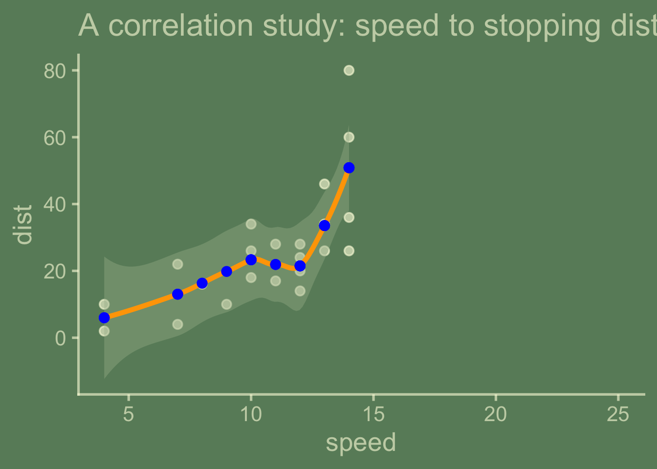
With subset of data, last_plot() %+% (cars |> filter(speed < 15))

change to teaching theme, last_plot() + ggchalkboard::theme_chalkboard()

1. Highlighting
2. Zooming
3. Panning

library(ggplot2); 
cars

# A tibble: 50 × 2
   speed  dist
   <dbl> <dbl>
 1     4     2
 2     4    10
 3     7     4
 4     7    22
 5     8    16
 6     9    10
 7    10    18
 8    10    26
 9    10    34
10    11    17
# ℹ 40 more rows

cars |>
ggplot(data = _) 

last_plot() + 
  aes(x = speed, y = dist)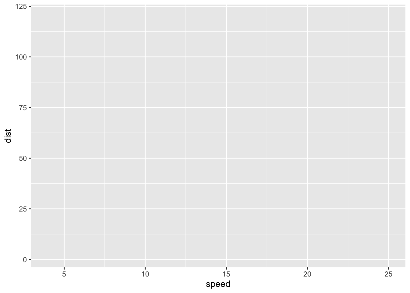

last_plot() + 
  geom_point()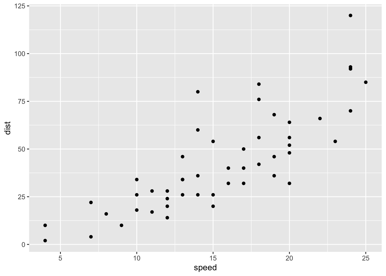

last_plot() + 
  labs(title = "A correlation study: speed to stopping distance")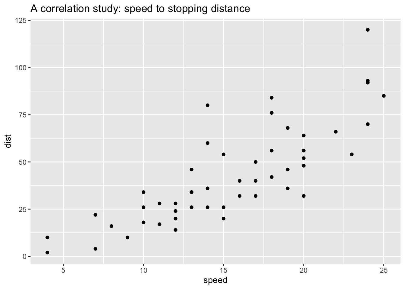

last_plot() + 
  geom_smooth()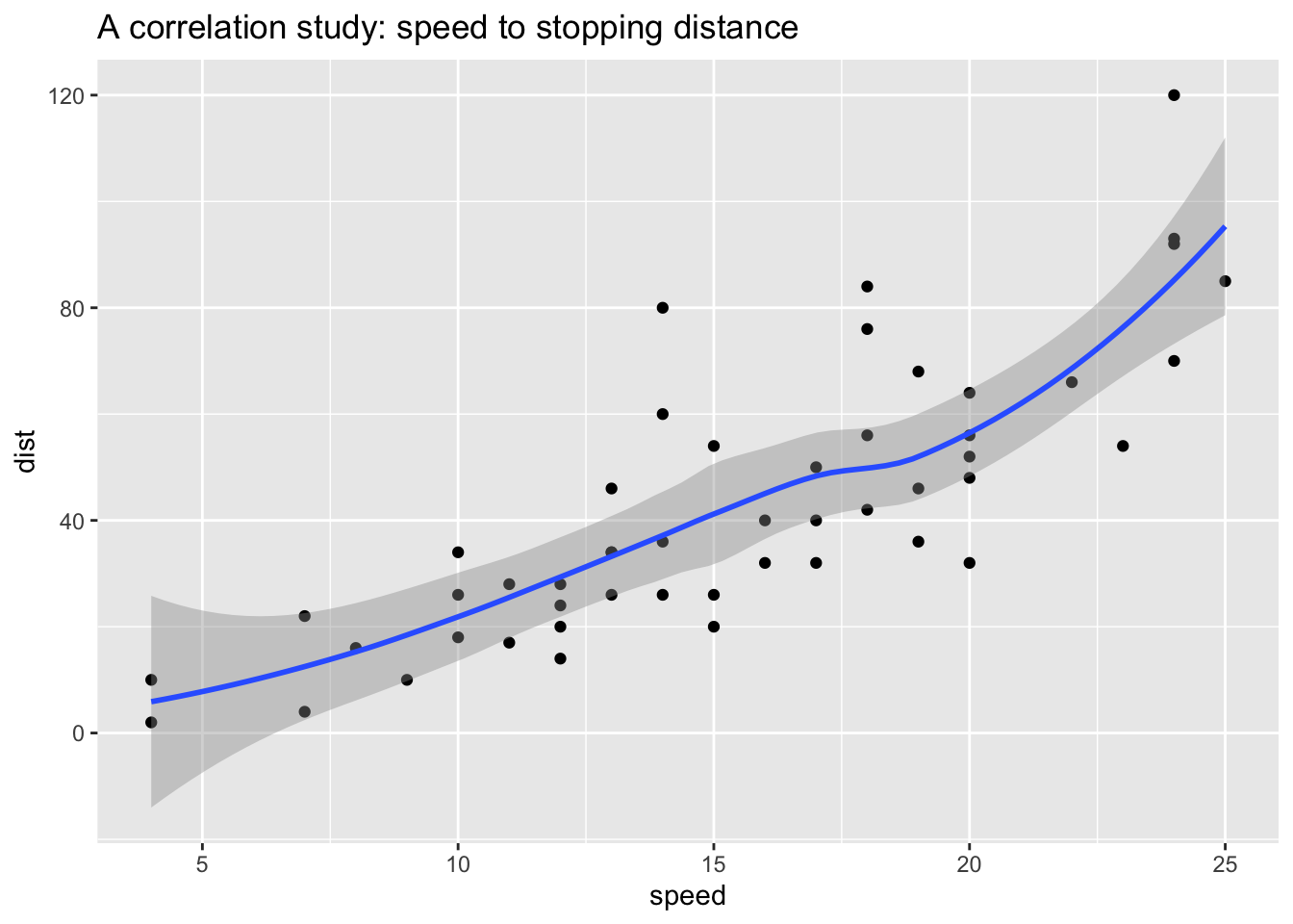

last_plot() + 
  stat_smooth(geom = GeomPoint, xseq = cars$speed, color = "blue")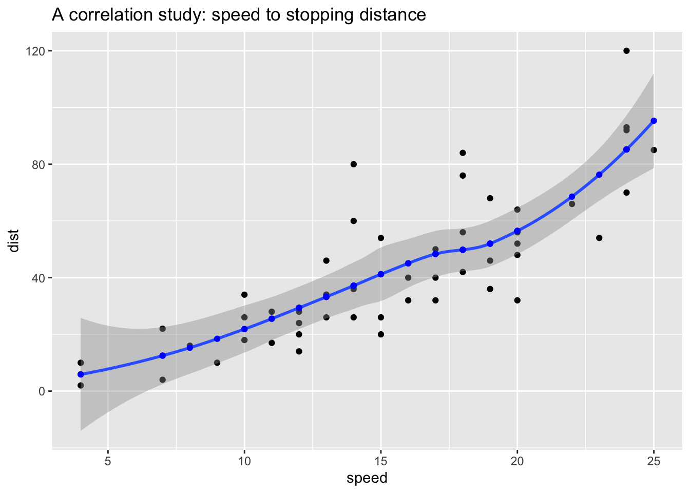

last_plot() %+%
  (cars |> filter(speed < 15))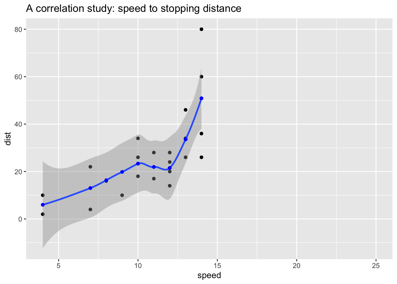

last_plot() +
  ggchalkboard::theme_chalkboard()