# 0. Use tidyverse
library(tidyverse)
# 1. define theme from convenience
# functions theme_grey, theme_classic
# theme_bw, etc.
theme_whitesmoke <- function(){
theme_bw(
base_size = 18,
base_family = "Times",
paper = "whitesmoke",
ink = "gray30",
accent = "magenta4")
}
# 2. set theme
theme_whitesmoke() |>
theme_set()
# 3. Get plotting!
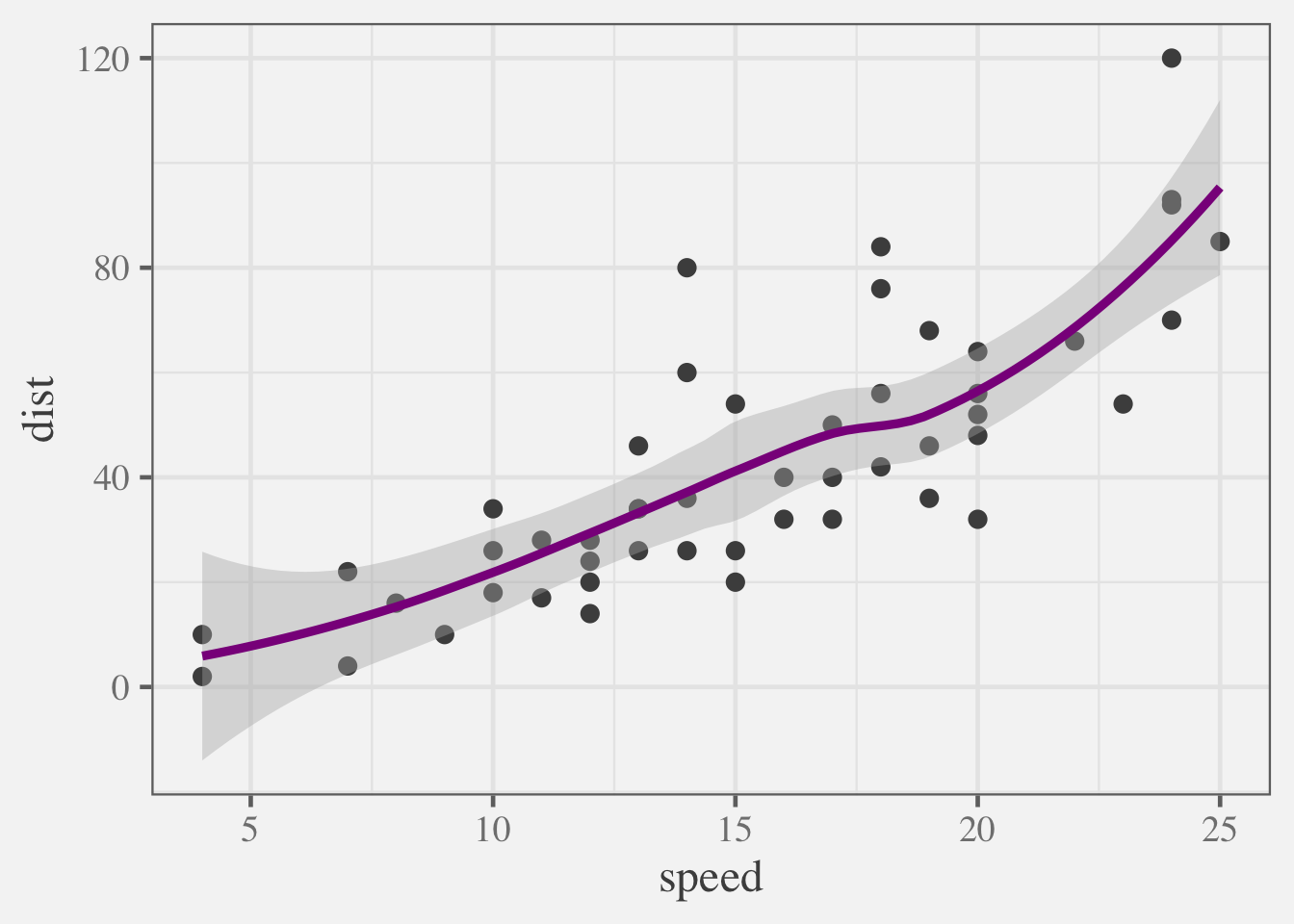
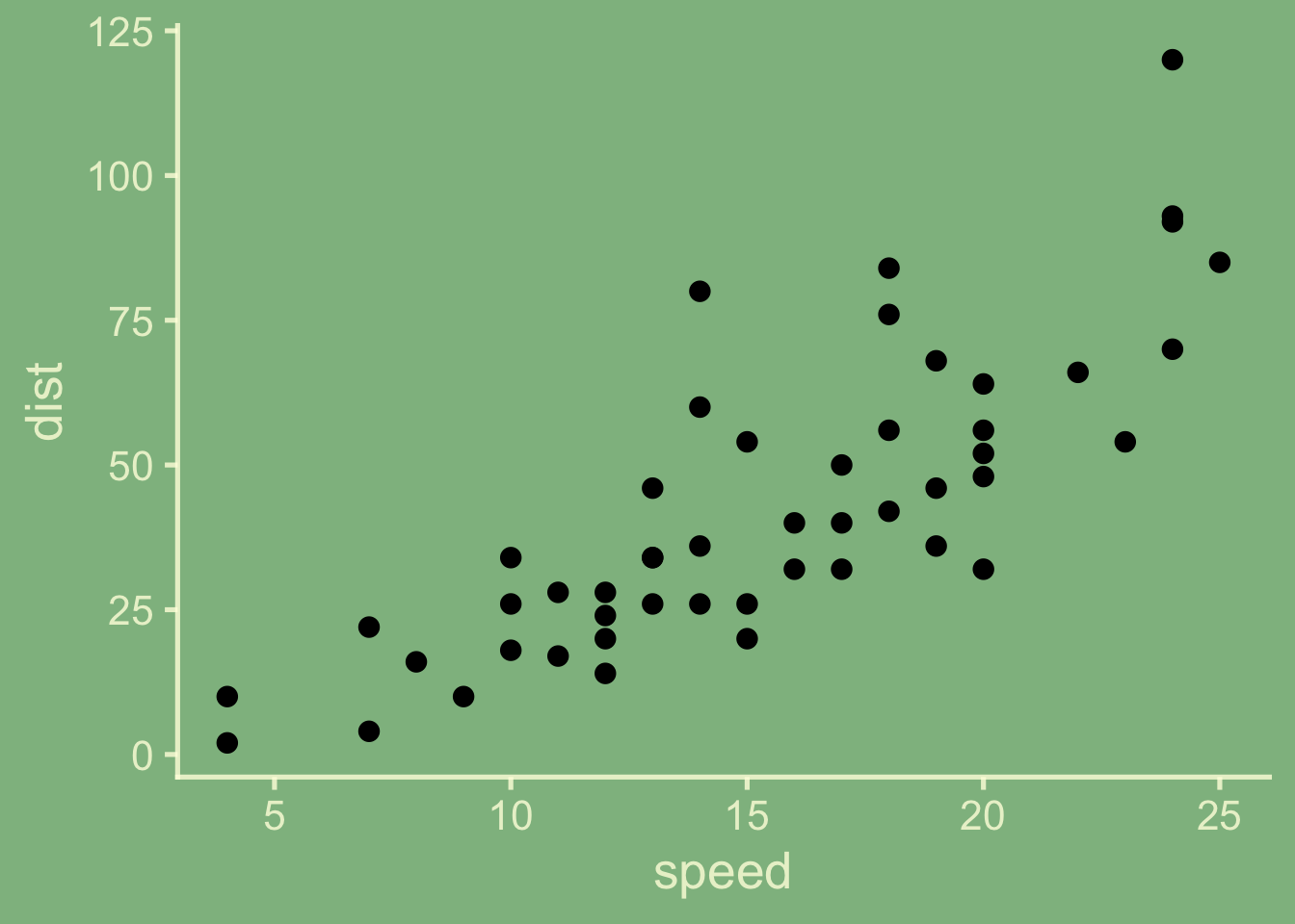
ggplot(data = cars) +
aes(x = speed, y = dist) +
geom_point() +
geom_smooth()
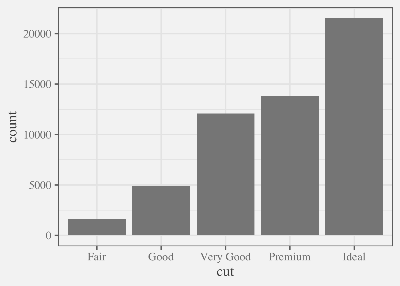
ggplot(data = diamonds) +
aes(x = cut) +
geom_bar()New ggplot2 theming will make plots extra sparkly ✨
And notes for using ggplot2 extensions that haven’t yet adopted dynamic geom_* theming
TLDR: The next release of ggplot2’s theming is something to be excited for!
A lot of value is delivered to analysts in the form of not needed to worry about fiddly details to adhering to brand theme – so we can focus more on the actual data analysis!
So the impactful innovations that are coming to ggplot2’s theming system are something to celebrate! (thanks to the creative vision of PR # and release ggplot2_3.5.2.9000 it’s nearly here! ) In our examples, we’ll celebrate new realities that we’re particularly excited for:
First, it’s never been easier to change the look and feel of your plot, as
paper,inkandaccentcolor governing arguments have been added to convenience functions liketheme_grey(),theme_classic(),theme_minimal()etc.Second,
geom_*()s (andstat_*()s) will be responsive to theme! Now, geom_ and stat_ layers should automatically take on the look and feel of your theme!
With these changes, you might be able to get to good enough when adhearing to brand theme with very little effort.
Radically change plot look and theme from convenience functions theme_grey(), theme_classic(), theme_minimal() etc.
Let’s see how new arguments paper, ink and accent in theming convenience functions theme_classic, theme_grey etc can dramatically change the look and feel of your plot! We’ll also use as old favorites like base_size and base_family.
In example A. we create the theme_whitesmoke – a modification of theme_classic. In example B. we create theme_chalkboard – a modification of theme_classic.
Example A. theme_whitesmoke
Example B. theme_chalkboard
For fun let’s also look at a more whimsical, classroom-inspired example.
# 1. define theme from convenience
# functions theme_grey, theme_classic
# theme_bw, etc.
theme_chalkboard <- function(){
  theme_classic(
         base_size = 20,
         paper = "darkseagreen",
         ink = alpha("lightyellow", .8),
         accent = alpha("orange", .8))
}

# 2. Set theme
theme_chalkboard() |>
  theme_set()

# 3. Get plotting!
ggplot(data = cars) +
  aes(x = speed, y = dist) +
  geom_point() +
  geom_smooth()

ggplot(data = diamonds) +
  aes(x = cut) +
  geom_bar()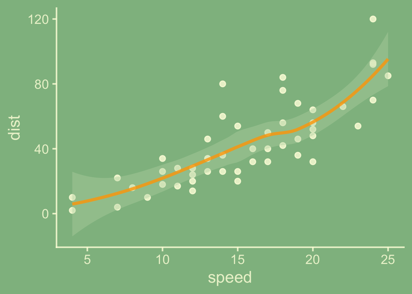
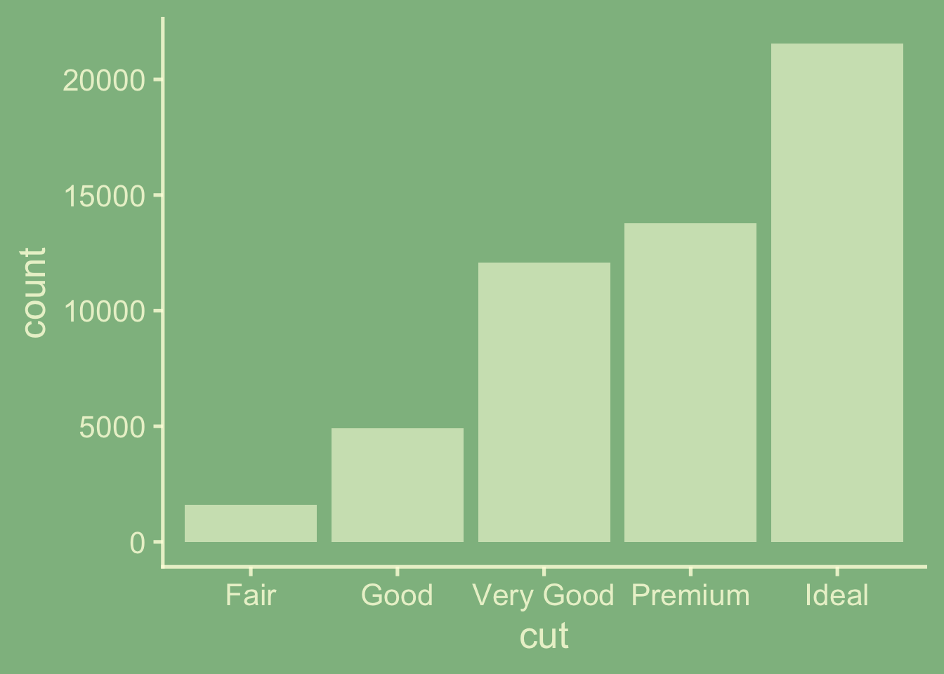
Are plots are classroom ready! And just so that we can appreciate the changes, without the new theming sytsem, you could define a theme that looked ‘chalkboardy’ with some effort, but the chalk (ink) wouldn’t automatically be used in the plotting space. So you’d get a visual like when setting or applying your theme, which leaves you asking ‘Who used a black sharpie on the chalkboard!?’:
But, what if my favorite geom_*() extension isn’t up-to-date with dynamic layer theming? How do I keep the chart to come into line with theme?
Unfortunate, ggplot2’s new theming won’t necessarily automatically benefit from the theming changes. Let’s have a look at this problem.
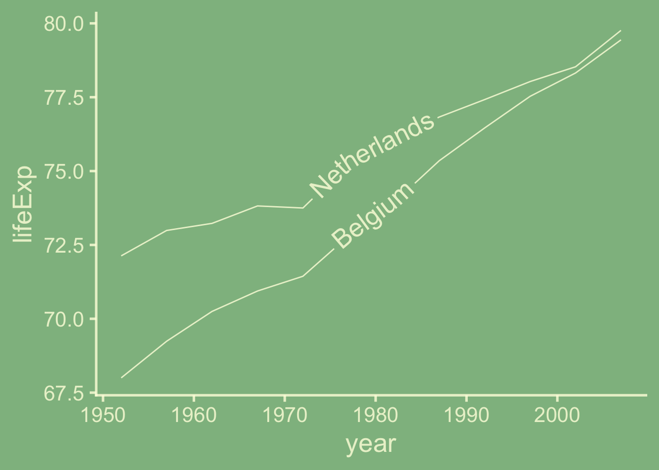
Problem: ggextension::geom_*() doesn’t dynamically theme.
As we see below
theme_chalkboard() |>
  theme_set()

two_countries <- gapminder::gapminder |>
  filter(country %in% c("Netherlands",
                        "Belgium"))

# Uh-oh! we see that geom_textpath has
# hardcoded set aesthetics
ggplot(data = two_countries) +
  aes(x = year,
      y = lifeExp,
      label = country) +
  geomtextpath::geom_textpath()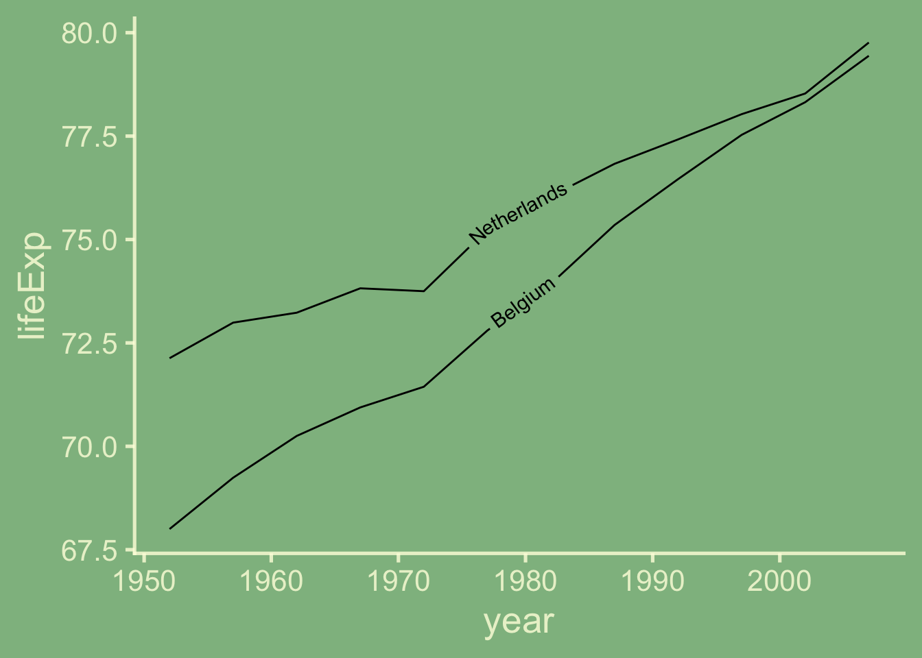
Solution i: Override defaults by naming colors/sizes that go with the theme
You can of course set geom_*() aesthetics in the usual way to get the layer to match the theme aesthetics, but you won’t scale
# Set defaults manually
ggplot(data = two_countries) +
  aes(x = year,
      y = lifeExp,
      label = country) +
  geomtextpath::geom_textpath(
    color = "lightyellow",
    size = 5
  )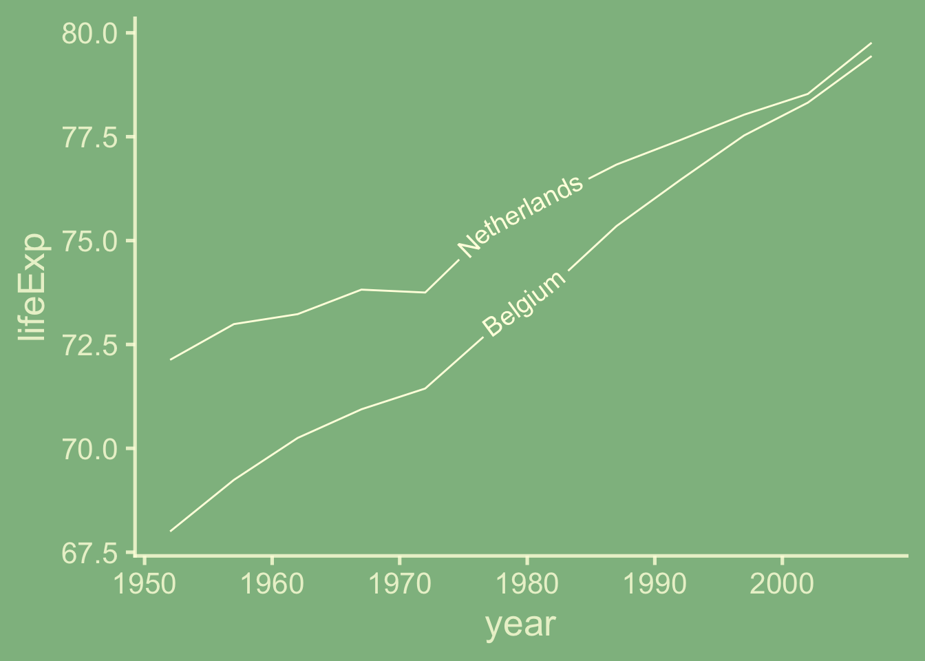
An more dynamic solution (ii): use aes(color = from_theme(ink), size = from_theme(fontsize))
Should you anticipate a possible change-up of your theme, you might use get_theme() instead of the name of the theme in the formulation above.
library(tidyverse)
theme_whitesmoke() |>
  theme_set()

ggplot(data = two_countries) +
  aes(x = year,
      y = lifeExp,
      label = country) +
  geomtextpath::geom_textpath(
    # set color, size from theme
    aes(color = from_theme(ink),
        size = from_theme(fontsize))
    )

# Set a new theme...
theme_chalkboard() |>
  theme_set()

# call plot again!
last_plot() 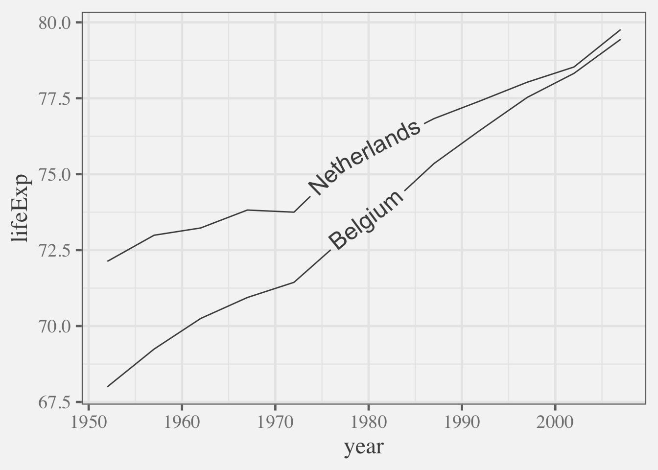
This method is also useful, if you want to adjust your plot keeping in harmony with theme settings.
library(ggplot2)

theme_bw(paper = "whitesmoke",
         ink = "grey25",
         base_size = 15) |>
  theme_set()

p <- ggplot(data = cars) +
  aes(x = speed,
      y = dist) +
  geom_line()

p1 <- p + geom_smooth()

p2 <- p +
  geom_smooth(aes(linewidth =
                    from_theme(linewidth)))

library(patchwork)
p1 + p2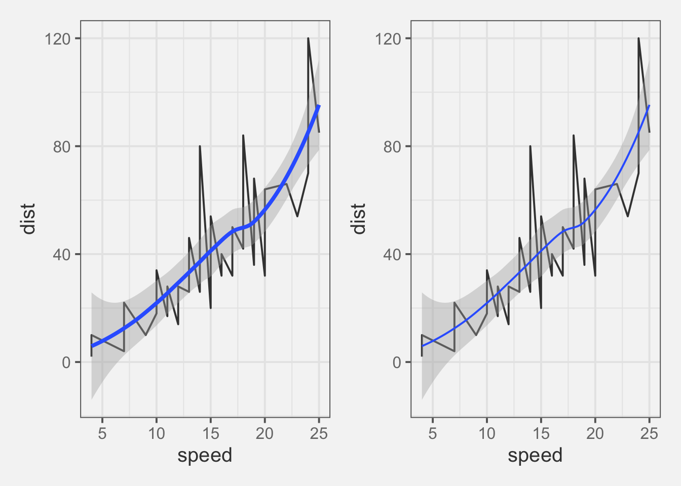
GeomSmooth$default_aes$linewidth<quosure>
expr: ^from_theme(2 * linewidth)
env: namespace:ggplot2theme_bw()$geom$linewidth[1] 0.5Curious about the evaluated theme values?
Although not a user-facing method.
theme_chalkboard()$geom$linewidth
theme_chalkboard()$geom$ink
theme_chalkboard()$geom$paper
[1] 0.9090909[1] "#FFFFE0CC"[1] "darkseagreen"End.
Are you an extender that needs to update your Geoms to take advantage of ggplot2’s new theming capabilities? Read on (maybe separate blog post)
—- Start new blog post… —-
Notes for Extenders: on writing layers that respond to theming declaration
There’s great news for extensions that define new layers that use Geoms from ‘base’ ggplot2 lock, stock and barrel - the dynamism will carry through to your layers if the new version of ggplot2 is loaded.
However, if you’ve created your own Geom object, you may have hard-coded default aesthetics. Color may be “black” and fill may be some shade of gray. This is modeled in the ggplot2 extension vignette geom_chull() example. Let’s have a look at that.
Your Geom may have hardcoded default aesthetics
Suppose you have created StatChull from the ggplot2 extension vignette, and have also created the modified GeomPolygon
# 1. Define compute
compute_group_chull <- function(data,
                                scales){

  row_num_convex_hull_members <-
    chull(x = data$x, y = data$y)

  data |>
    slice(row_num_convex_hull_members)

}

# 2. Define Stat
StatChull <- ggproto(
  `_class` = "StatChull",
  `_inherit` = Stat,
  required_aes = c("x", "y"),
  compute_group = compute_group_chull
  )
# 3. Define Geom: Modified GeomPolygon
GeomPolygonHollow <-
ggproto("GeomPolygonHollow",
GeomPolygon,
default_aes =
aes(colour = "black",
fill = NA,
linewidth = 0.5,
linetype = 1,
alpha = NA)
)
# 4. Test Geom X Stat w/ theme
theme_chalkboard() |>
theme_set()
ggplot(mtcars) +
aes(x = drat, y = wt) +
geom_point() +
layer(stat = StatChull,
geom = GeomPolygonHollow,
position = position_identity())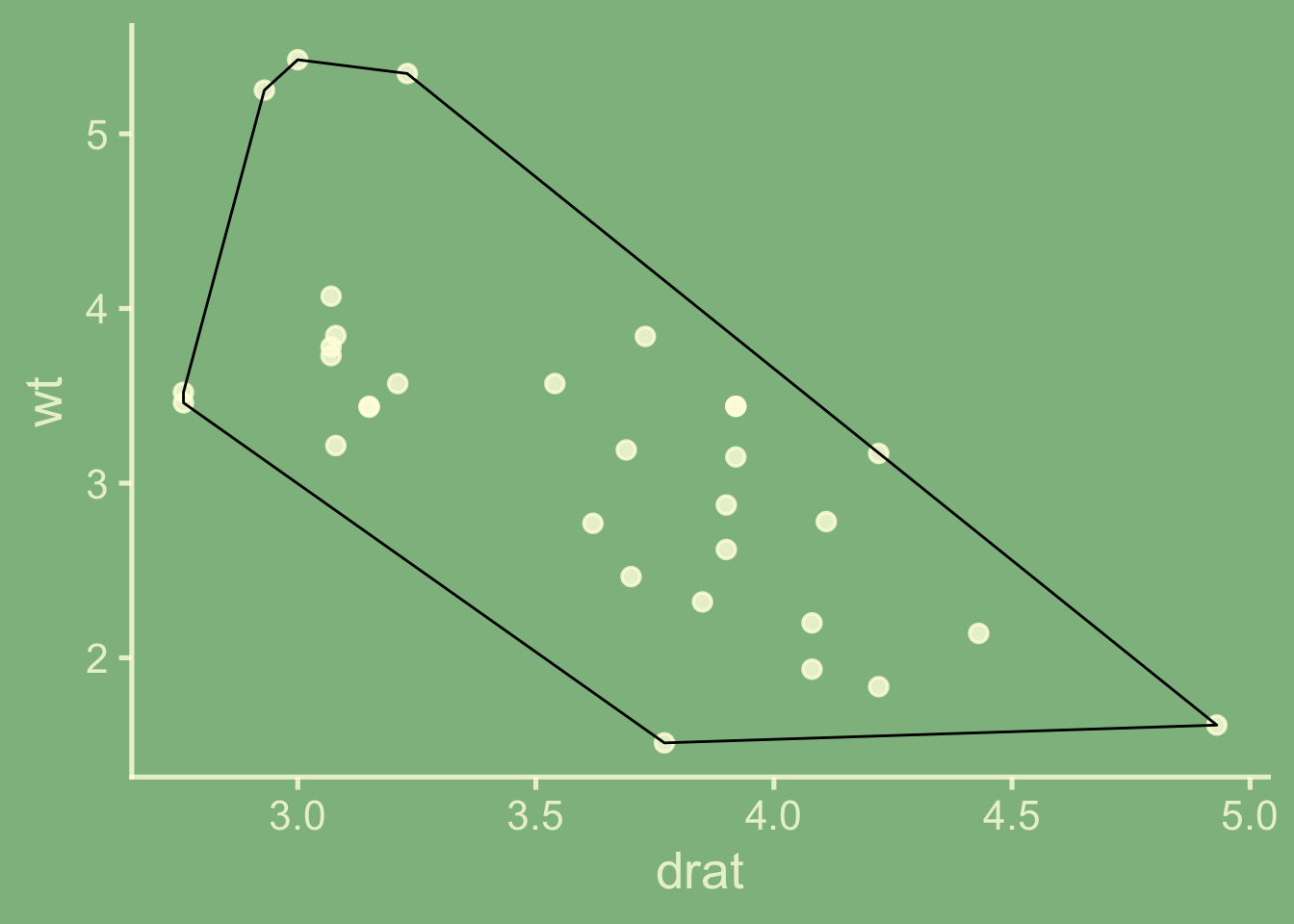
But, if we look at the definition of GeomPolygon in the latest ggplot2 development version, we see default aesthetics are no longer hardcoded, which is what allows our layers to be themed.
GeomPolygon$default_aesAesthetic mapping:
* `colour` -> `from_theme(colour %||% NA)`
* `fill` -> `from_theme(fill %||% col_mix(ink, paper, 0.2))`
* `linewidth` -> `from_theme(borderwidth)`
* `linetype` -> `from_theme(bordertype)`
* `alpha` -> NA
* `subgroup` -> NULLUse piggy back on default aesthetics of ‘base’ ggplot2 Geoms, to inherit dynamism (and get backward compatiblity for free!).
For extenders, there are a few ways to update Geom default aes so that they take on characteristics specified by theme.
# 1. determine aesthetics that need defaults
GeomPolygon$default_aes
Aesthetic mapping:
* `colour` -> `from_theme(colour %||% NA)`
* `fill` -> `from_theme(fill %||% col_mix(ink, paper, 0.2))`
* `linewidth` -> `from_theme(borderwidth)`
* `linetype` -> `from_theme(bordertype)`
* `alpha` -> NA
* `subgroup` -> NULL# Update create GeomPolygonHollow to have
# GeomLine defaults and fill = NA
GeomPolygonHollow <-
ggproto(`_class` = "GeomPolygonHollow",
`_inherit` = GeomPolygon,
default_aes =
GeomPolygon$default_aes |>
modifyList(GeomLine$default_aes) |>
modifyList(aes(fill = NA))
)# 2. inspect newly defined aesthetics
GeomPolygonHollow$default_aes
# 3. Try out GeomPolygonHollow
ggplot(mtcars) +
aes(x = drat,
y = wt) +
geom_point() +
layer(stat = StatChull,
geom = GeomPolygonHollow,
position = "identity")Aesthetic mapping:
* `colour` -> `from_theme(colour %||% ink)`
* `fill` -> NA
* `linewidth` -> `from_theme(linewidth)`
* `linetype` -> `from_theme(linetype)`
* `alpha` -> NA
* `subgroup` -> NULL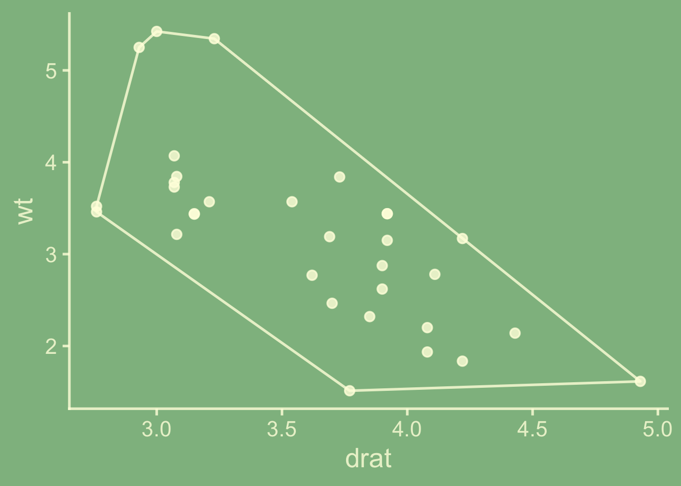
To write: ‘wait until 4.0.0 is released and bump your required ggplot2 version’
To write: Or use onLoad for backward compatibility
To be written up… > another way is described in PR ggforce
End blog post for extenders…
knitr::knit_exit()