class: inverse, bottom background-image: url(https://images.unsplash.com/photo-1588591795084-1770cb3be374?q=80&w=2070&auto=format&fit=crop&ixlib=rb-4.1.0&ixid=M3wxMjA3fDB8MHxwaG90by1wYWdlfHx8fGVufDB8fHx8fA%3D%3D) background-size: cover ## .large[R Medicine 2026: ggregions for building intuitive coding interfaces for anatomical visualizations] ## .small[] #### .tiny[Dr. Evangeline Reynolds | 2026-05-01 | DU, Image credit: Ross Sneddon, Upsplash] ??? Title slide --- class: inverse # Motivations for ggregions > ### I am told there are people who do not care for maps, and I find it hard to believe. - Robert Louis Stevenson -- > ### 'My teacher, Mr. Jayson, says a map is a picture of someplace from above. It's like flying over that spot in an airplane.' - 'Lisa' in Loreen Leedy's in 'Mappying Penny's World' --- # But ... > ### I hate when I work with spatial data that so much of my mindshare goes to thinking about 'how do I wrangle this map and what on earth is going on' versus the actual meaning behind what I'm trying to map. - Emily Riederer --- class: inverse -- ## There is great support for mapping in R and in the data visualization library {ggplot2} which supports many R packages. -- ## But, producing a simple map, like a choropleth, can feel much harder than producing other plots, like a scatterplot for example in ggplot2. --- count: false .panel1-classic_v_semantic-auto[ ``` r *tribble(~var1, ~var2, ~var3, * 1, 4, T, * 2, 3, F) ``` ] .panel2-classic_v_semantic-auto[ ``` # A tibble: 2 × 3 var1 var2 var3 <dbl> <dbl> <lgl> 1 1 4 TRUE 2 2 3 FALSE ``` ] --- count: false .panel1-classic_v_semantic-auto[ ``` r tribble(~var1, ~var2, ~var3, 1, 4, T, 2, 3, F) |> * ggplot() ``` ] .panel2-classic_v_semantic-auto[ <!-- --> ] --- count: false .panel1-classic_v_semantic-auto[ ``` r tribble(~var1, ~var2, ~var3, 1, 4, T, 2, 3, F) |> ggplot() + * aes(x = var1, * y = var2) ``` ] .panel2-classic_v_semantic-auto[ <!-- --> ] --- count: false .panel1-classic_v_semantic-auto[ ``` r tribble(~var1, ~var2, ~var3, 1, 4, T, 2, 3, F) |> ggplot() + aes(x = var1, y = var2) + * geom_point(size = 4) ``` ] .panel2-classic_v_semantic-auto[ <!-- --> ] --- count: false .panel1-classic_v_semantic-auto[ ``` r tribble(~var1, ~var2, ~var3, 1, 4, T, 2, 3, F) |> ggplot() + aes(x = var1, y = var2) + geom_point(size = 4) + * aes(color = var3) ``` ] .panel2-classic_v_semantic-auto[ <!-- --> ] <style> .panel1-classic_v_semantic-auto { color: black; width: 38.6060606060606%; hight: 32%; float: left; padding-left: 1%; font-size: 80% } .panel2-classic_v_semantic-auto { color: black; width: 59.3939393939394%; hight: 32%; float: left; padding-left: 1%; font-size: 80% } .panel3-classic_v_semantic-auto { color: black; width: NA%; hight: 33%; float: left; padding-left: 1%; font-size: 80% } </style> --- count: false .panel1-semantic-auto[ ``` r *tribble(~place, ~var2, * "Texas", T, * "Indiana", F) ``` ] .panel2-semantic-auto[ ``` # A tibble: 2 × 2 place var2 <chr> <lgl> 1 Texas TRUE 2 Indiana FALSE ``` ] --- count: false .panel1-semantic-auto[ ``` r tribble(~place, ~var2, "Texas", T, "Indiana", F) |> *ggplot() ``` ] .panel2-semantic-auto[ <!-- --> ] --- count: false .panel1-semantic-auto[ ``` r tribble(~place, ~var2, "Texas", T, "Indiana", F) |> ggplot() + * aes(state_name = place) ``` ] .panel2-semantic-auto[ <!-- --> ] --- count: false .panel1-semantic-auto[ ``` r tribble(~place, ~var2, "Texas", T, "Indiana", F) |> ggplot() + aes(state_name = place) + * geom_state() ``` ] .panel2-semantic-auto[ <!-- --> ] --- count: false .panel1-semantic-auto[ ``` r tribble(~place, ~var2, "Texas", T, "Indiana", F) |> ggplot() + aes(state_name = place) + geom_state() + * aes(fill = var2) ``` ] .panel2-semantic-auto[ <!-- --> ] <style> .panel1-semantic-auto { color: black; width: 38.6060606060606%; hight: 32%; float: left; padding-left: 1%; font-size: 80% } .panel2-semantic-auto { color: black; width: 59.3939393939394%; hight: 32%; float: left; padding-left: 1%; font-size: 80% } .panel3-semantic-auto { color: black; width: NA%; hight: 33%; float: left; padding-left: 1%; font-size: 80% } </style> --- class: inverse ## Semantic -- ## Positional -- ## Encoding --- class: inverse ## Semantic (*meaning* of words or symbols) ## Positional ## Encoding -- ### 'normal' ggplot2 positional encoding -- ### `aes(x = c(1, 2), y = c(4, 2))` -- ### S.P.E. -- ### `aes(state_name = c("Texas", "Indiana"))` <!-- #### ggregions posits that by investing in methods to easily create new geo-specific ggplot2 layer extensions (geom_*s), producing maps with ggplot2 can become as intuitive as creating other plots. About specifying a map, you might say, 'use this data, draw regions, position and color fill according to var1 and var2.' --> <!-- The proposed regions mapping might look something like this: --> --- class: inverse, center, middle # Does {ggregions} deliver? --- count: false .panel1-usmapdata0-auto[ ``` r *library(ggplot2) ``` ] .panel2-usmapdata0-auto[ ] --- count: false .panel1-usmapdata0-auto[ ``` r library(ggplot2) *us_income ``` ] .panel2-usmapdata0-auto[ ``` # A tibble: 52 × 5 GEOID NAME variable income moe <chr> <chr> <chr> <dbl> <dbl> 1 01 Alabama income 24476 136 2 02 Alaska income 32940 508 3 04 Arizona income 27517 148 4 05 Arkansas income 23789 165 5 06 California income 29454 109 6 08 Colorado income 32401 109 7 09 Connecticut income 35326 195 8 10 Delaware income 31560 247 9 11 District of Columbia income 43198 681 10 12 Florida income 25952 70 # ℹ 42 more rows ``` ] --- count: false .panel1-usmapdata0-auto[ ``` r library(ggplot2) us_income |> * ggplot() ``` ] .panel2-usmapdata0-auto[ <!-- --> ] --- count: false .panel1-usmapdata0-auto[ ``` r library(ggplot2) us_income |> ggplot() + * aes(state_name = NAME) ``` ] .panel2-usmapdata0-auto[ <!-- --> ] --- count: false .panel1-usmapdata0-auto[ ``` r library(ggplot2) us_income |> ggplot() + aes(state_name = NAME) + * geom_state() ``` ] .panel2-usmapdata0-auto[ <!-- --> ] --- count: false .panel1-usmapdata0-auto[ ``` r library(ggplot2) us_income |> ggplot() + aes(state_name = NAME) + geom_state() + * aes(fill = income) ``` ] .panel2-usmapdata0-auto[ <!-- --> ] <style> .panel1-usmapdata0-auto { color: black; width: 38.6060606060606%; hight: 32%; float: left; padding-left: 1%; font-size: 80% } .panel2-usmapdata0-auto { color: black; width: 59.3939393939394%; hight: 32%; float: left; padding-left: 1%; font-size: 80% } .panel3-usmapdata0-auto { color: black; width: NA%; hight: 33%; float: left; padding-left: 1%; font-size: 80% } </style> --- > ## [ggregions-generated] APIs feels like they actually puts the "question" at the center. - Emily Riederer --- class: inverse, center, middle # How does it work? --- ## Effortlessly write new region-specific geom_* functions. <!-- The {ggregions} allows API creators to quickly create easy-to-use ggplot2 layer extensions (e.g. geom_*()s) that adhere to the ggplot2 'grammar'. --> --- --- count: false ## Example with geographic regions: US states ### Step 1. prepare data .panel1-us_states_ref-auto[ ``` r *library(dplyr) ``` ] .panel2-us_states_ref-auto[ ] --- count: false ## Example with geographic regions: US states ### Step 1. prepare data .panel1-us_states_ref-auto[ ``` r library(dplyr) # Step 1. prep some of their geo reference data *usmapdata::us_map() ``` ] .panel2-us_states_ref-auto[ ``` Simple feature collection with 52 features and 3 fields Geometry type: MULTIPOLYGON Dimension: XY Bounding box: xmin: -2584074 ymin: -2602555 xmax: 2516258 ymax: 731628.1 Projected CRS: NAD27 / US National Atlas Equal Area First 10 features: fips abbr full geom 1 02 AK Alaska MULTIPOLYGON (((-2390688 -2... 2 01 AL Alabama MULTIPOLYGON (((1091785 -13... 3 05 AR Arkansas MULTIPOLYGON (((482022.2 -9... 4 04 AZ Arizona MULTIPOLYGON (((-1386064 -1... 5 06 CA California MULTIPOLYGON (((-1716581 -1... 6 08 CO Colorado MULTIPOLYGON (((-787705.6 -... 7 09 CT Connecticut MULTIPOLYGON (((2156162 -83... 8 11 DC District of Columbia MULTIPOLYGON (((1950799 -40... 9 10 DE Delaware MULTIPOLYGON (((2037480 -28... 10 12 FL Florida MULTIPOLYGON (((1853163 -20... ``` ] --- count: false ## Example with geographic regions: US states ### Step 1. prepare data .panel1-us_states_ref-auto[ ``` r library(dplyr) # Step 1. prep some of their geo reference data usmapdata::us_map() |> * select(state_name = full, * state_abbr = abbr, * state_fips = fips, * geometry = geom) ``` ] .panel2-us_states_ref-auto[ ``` Simple feature collection with 52 features and 3 fields Geometry type: MULTIPOLYGON Dimension: XY Bounding box: xmin: -2584074 ymin: -2602555 xmax: 2516258 ymax: 731628.1 Projected CRS: NAD27 / US National Atlas Equal Area First 10 features: state_name state_abbr state_fips geometry 1 Alaska AK 02 MULTIPOLYGON (((-2390688 -2... 2 Alabama AL 01 MULTIPOLYGON (((1091785 -13... 3 Arkansas AR 05 MULTIPOLYGON (((482022.2 -9... 4 Arizona AZ 04 MULTIPOLYGON (((-1386064 -1... 5 California CA 06 MULTIPOLYGON (((-1716581 -1... 6 Colorado CO 08 MULTIPOLYGON (((-787705.6 -... 7 Connecticut CT 09 MULTIPOLYGON (((2156162 -83... 8 District of Columbia DC 11 MULTIPOLYGON (((1950799 -40... 9 Delaware DE 10 MULTIPOLYGON (((2037480 -28... 10 Florida FL 12 MULTIPOLYGON (((1853163 -20... ``` ] --- count: false ## Example with geographic regions: US states ### Step 1. prepare data .panel1-us_states_ref-auto[ ``` r library(dplyr) # Step 1. prep some of their geo reference data usmapdata::us_map() |> select(state_name = full, state_abbr = abbr, state_fips = fips, geometry = geom) -> *us_states_ref ``` ] .panel2-us_states_ref-auto[ ] <style> .panel1-us_states_ref-auto { color: black; width: 38.6060606060606%; hight: 32%; float: left; padding-left: 1%; font-size: 80% } .panel2-us_states_ref-auto { color: black; width: 59.3939393939394%; hight: 32%; float: left; padding-left: 1%; font-size: 80% } .panel3-us_states_ref-auto { color: black; width: NA%; hight: 33%; float: left; padding-left: 1%; font-size: 80% } </style> --- ### Step 2. write user-facing functions with ggregion 'write' utilities <!-- Then, authors will be able use `write_geom_region()` to create a regions-specific ggplot2 layer, for example `geom_state()` below, which can be made available in their geo packages. --> ``` r library(ggregions) geom_state <- write_geom_region(us_states_ref, required_aes = "state_name|state_abbr|state_fips") stamp_state <- write_stamp_region(us_states_ref, required_aes = "state_name|state_abbr|state_fips") geom_state_text <- write_geom_region_text(us_states_ref, required_aes = "state_name|state_abbr|state_fips") stamp_state_text <- write_stamp_region_text(us_states_ref, required_aes = "state_name|state_abbr|state_fips") ``` --- ### Step 2b. (optional) Inspect user-facing function ``` r geom_state ``` ``` function (mapping = aes(), data = NULL, stat = StatRegion, position = "identity", na.rm = FALSE, show.legend = NA, inherit.aes = TRUE, ref_data = us_states_ref, ...) { c(layer_sf(geom = GeomSf, data = data, mapping = mapping, stat = stat, position = position, show.legend = show.legend, inherit.aes = inherit.aes, params = rlang::list2(na.rm = na.rm, ref_data = ref_data, ...)), coord_sf(crs = st_crs_mod(ref_data))) } <environment: namespace:ggregions> ``` --- #### Steb 2bb (for the truely curious) Inspect StatRegions compute ``` r ggregions:::StatRegion$compute_panel ``` ``` <ggproto method> <Wrapper function> function (...) compute_panel(...) <Inner function (f)> function (data, scales, ref_data, keep = NULL, drop = NULL, stamp = F) { ref_data$id <- ref_data[1][[1]] if (!is.null(keep)) { ref_data <- dplyr::filter(ref_data, id %in% keep) } if (!is.null(drop)) { ref_data <- dplyr::filter(ref_data, !(id %in% drop)) } ref_data <- ggplot2::StatSfCoordinates$compute_group(ggplot2::StatSf$compute_panel(ref_data, coord = ggplot2::CoordSf), coord = ggplot2::CoordSf) if (!stamp) { dplyr::inner_join(ref_data, data) } else { ref_data } } ``` --- ### What does `ggregions::write_geom_region()` do? ``` r ggregions::write_geom_region ``` ``` function (ref_data = australia_state_ref, required_aes = NULL) { modified_fun <- geom_region formals(modified_fun)$ref_data <- substitute(ref_data) return(modified_fun) } <bytecode: 0x10b4698a8> <environment: namespace:ggregions> ``` -- ``` r ggregions:::geom_region ``` ``` function (mapping = aes(), data = NULL, stat = StatRegion, position = "identity", na.rm = FALSE, show.legend = NA, inherit.aes = TRUE, ref_data, ...) { c(layer_sf(geom = GeomSf, data = data, mapping = mapping, stat = stat, position = position, show.legend = show.legend, inherit.aes = inherit.aes, params = rlang::list2(na.rm = na.rm, ref_data = ref_data, ...)), coord_sf(crs = st_crs_mod(ref_data))) } <bytecode: 0x10b46c4b0> <environment: namespace:ggregions> ``` <!-- ## Deliver intuitive, newcomer-welcoming spatial viz experience --> <!-- By including the newly specified `geom_` function in their geo data package (perhaps instead or in addition to a convenience wrapper that are typical of geo packages) the package *users* will be able to use the` data + aes + geom` formulation for defining their plots. Instead of positional aesthetics like x, y or geometry, a region identifier like `state_name` or `fips` can be used. Internally, the regions `geom_*` will translate between place name or other identifier to the necessary borders (`sfc`s). --> <!-- Below is some tabular data with geographic region identifiers, but no boundaries: --> <!-- Even though there is no boundary information, analysts can map this data with the familiar data + aesthetic mapping + layer syntax that makes ggplot2 easy to read, write, and reason about. --> --- count: false .panel1-usmapdata-auto[ ``` r *library(ggplot2) ``` ] .panel2-usmapdata-auto[ ] --- count: false .panel1-usmapdata-auto[ ``` r library(ggplot2) *library(usmapdata) ``` ] .panel2-usmapdata-auto[ ] --- count: false .panel1-usmapdata-auto[ ``` r library(ggplot2) library(usmapdata) *us_income ``` ] .panel2-usmapdata-auto[ ``` # A tibble: 52 × 5 GEOID NAME variable income moe <chr> <chr> <chr> <dbl> <dbl> 1 01 Alabama income 24476 136 2 02 Alaska income 32940 508 3 04 Arizona income 27517 148 4 05 Arkansas income 23789 165 5 06 California income 29454 109 6 08 Colorado income 32401 109 7 09 Connecticut income 35326 195 8 10 Delaware income 31560 247 9 11 District of Columbia income 43198 681 10 12 Florida income 25952 70 # ℹ 42 more rows ``` ] --- count: false .panel1-usmapdata-auto[ ``` r library(ggplot2) library(usmapdata) us_income |> * ggplot() ``` ] .panel2-usmapdata-auto[ <!-- --> ] --- count: false .panel1-usmapdata-auto[ ``` r library(ggplot2) library(usmapdata) us_income |> ggplot() + * aes(state_name = NAME) ``` ] .panel2-usmapdata-auto[ <!-- --> ] --- count: false .panel1-usmapdata-auto[ ``` r library(ggplot2) library(usmapdata) us_income |> ggplot() + aes(state_name = NAME) + * geom_state() ``` ] .panel2-usmapdata-auto[ <!-- --> ] --- count: false .panel1-usmapdata-auto[ ``` r library(ggplot2) library(usmapdata) us_income |> ggplot() + aes(state_name = NAME) + geom_state() + * aes(fill = income) ``` ] .panel2-usmapdata-auto[ <!-- --> ] --- count: false .panel1-usmapdata-auto[ ``` r library(ggplot2) library(usmapdata) us_income |> ggplot() + aes(state_name = NAME) + geom_state() + aes(fill = income) + * scale_fill_viridis_c(option = "magma") ``` ] .panel2-usmapdata-auto[ <!-- --> ] --- count: false .panel1-usmapdata-auto[ ``` r library(ggplot2) library(usmapdata) us_income |> ggplot() + aes(state_name = NAME) + geom_state() + aes(fill = income) + scale_fill_viridis_c(option = "magma") + * geom_state_text(color = "white") ``` ] .panel2-usmapdata-auto[ <!-- --> ] --- count: false .panel1-usmapdata-auto[ ``` r library(ggplot2) library(usmapdata) us_income |> ggplot() + aes(state_name = NAME) + geom_state() + aes(fill = income) + scale_fill_viridis_c(option = "magma") + geom_state_text(color = "white") + * aes(label = after_stat(state_abbr)) ``` ] .panel2-usmapdata-auto[ 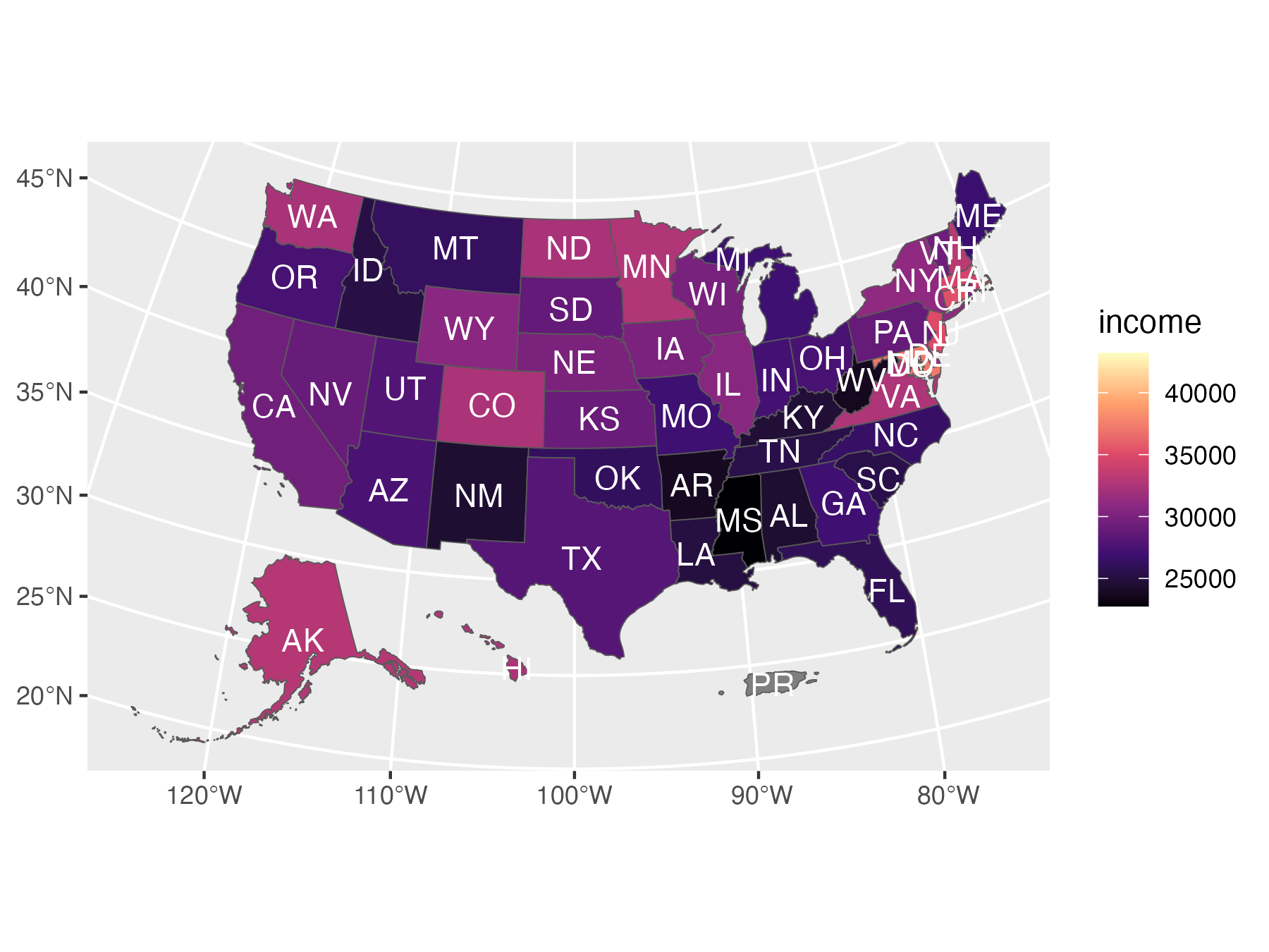<!-- --> ] <style> .panel1-usmapdata-auto { color: black; width: 38.6060606060606%; hight: 32%; float: left; padding-left: 1%; font-size: 80% } .panel2-usmapdata-auto { color: black; width: 59.3939393939394%; hight: 32%; float: left; padding-left: 1%; font-size: 80% } .panel3-usmapdata-auto { color: black; width: NA%; hight: 33%; float: left; padding-left: 1%; font-size: 80% } </style> <!-- Packages that might take avantage of ggregion's functionality include --> <!-- [afrimapr](https://afrimapr.github.io/afrimapr.website/), [geobr](https://ipeagit.github.io/geobr/), [cancensus](https://mountainmath.github.io/cancensus/index.html), [chilemapas](https://pacha.dev/chilemapas/), [RCzechia](https://github.com/jlacko/RCzechia), [geofi](https://ropengov.github.io/geofi/) --> <!-- , [geokz](https://github.com/arodionoff/geokz), [mapsPERU](https://github.com/musajajorge/mapsPERU) and [geoidep](https://geografo.pe/geoidep/index.html), [mapSpain](https://github.com/rOpenSpain/mapSpain/), [geographr](https://github.com/britishredcrosssociety/geographr), [geouy](https://github.com/RichDeto/geouy), [tigris](https://github.com/walkerke/tigris), --> <!-- and [rgeoboundaries](https://github.com/wmgeolab/rgeoboundaries). --> <!-- Since these geo packages have many users, the impacts of `{ggregions}` could be significant. --> --- class: inverse, center, middle # Anatomical regions --- ### ggregions with teethr::dental_arcade_mapping https://github.com/bbartholdy/teethr --- ### data preparation ``` r teethr::dental_arcade_mapping |> as_tibble() |> left_join(teethr::tooth_notation |> rename(tooth = text)) |> select(tooth_id = tooth, fdi = FDI, standard = standards, geometry) -> teeth_ref_data ``` -- ### ggplot2 'layer' preparation ``` r library(ggregions) geom_tooth <- write_geom_region(teeth_ref_data, required_aes = "tooth_id|fdi|standard") geom_tooth_text <- write_geom_region_text(teeth_ref_data, required_aes = "tooth_id|fdi|standard") stamp_tooth <- write_stamp_region(teeth_ref_data, required_aes = "tooth_id|fdi|standard") stamp_tooth_text <- write_stamp_region_text(teeth_ref_data, required_aes = "tooth_id|fdi|standard") ``` --- count: false ### yields user-friendly API .panel1-arcade-auto[ ``` r *caries_ratios ``` ] .panel2-arcade-auto[ ``` # A tibble: 32 × 4 tooth n count ratio <chr> <int> <dbl> <dbl> 1 URI1 35 4 0.114 2 URI2 31 4 0.129 3 URC1 35 7 0.2 4 URP1 34 3 0.0882 5 URP2 23 5 0.217 6 URM1 32 7 0.219 7 URM2 25 7 0.28 8 URM3 22 9 0.409 9 ULI1 28 2 0.0714 10 ULI2 26 2 0.0769 # ℹ 22 more rows ``` ] --- count: false ### yields user-friendly API .panel1-arcade-auto[ ``` r caries_ratios |> * ggplot() ``` ] .panel2-arcade-auto[ <!-- --> ] --- count: false ### yields user-friendly API .panel1-arcade-auto[ ``` r caries_ratios |> ggplot() + * aes(tooth_id = tooth, * fill = ratio) ``` ] .panel2-arcade-auto[ <!-- --> ] --- count: false ### yields user-friendly API .panel1-arcade-auto[ ``` r caries_ratios |> ggplot() + aes(tooth_id = tooth, fill = ratio) + * geom_tooth(alpha = .5) ``` ] .panel2-arcade-auto[ <!-- --> ] --- count: false ### yields user-friendly API .panel1-arcade-auto[ ``` r caries_ratios |> ggplot() + aes(tooth_id = tooth, fill = ratio) + geom_tooth(alpha = .5) + * stamp_tooth_text(size = 2) ``` ] .panel2-arcade-auto[ <!-- --> ] --- count: false ### yields user-friendly API .panel1-arcade-auto[ ``` r caries_ratios |> ggplot() + aes(tooth_id = tooth, fill = ratio) + geom_tooth(alpha = .5) + stamp_tooth_text(size = 2) + * scale_fill_viridis_c() ``` ] .panel2-arcade-auto[ <!-- --> ] <style> .panel1-arcade-auto { color: black; width: 38.6060606060606%; hight: 32%; float: left; padding-left: 1%; font-size: 80% } .panel2-arcade-auto { color: black; width: 59.3939393939394%; hight: 32%; float: left; padding-left: 1%; font-size: 80% } .panel3-arcade-auto { color: black; width: NA%; hight: 33%; float: left; padding-left: 1%; font-size: 80% } </style> --- <img src="r-medicine-ggregions_files/figure-html/unnamed-chunk-13-1.png" width="65%" /> --- ## ggregions X gganatogram::hgFemale_list ### Step 1: Data preparation ``` r female_sf <- gganatogram::hgFemale_list[c(1:156, 180:195)] |> # return to this!! bind_rows() |> remove_missing() |> to_sf_routine() ref_female_sf <- female_sf |> select(organ = id, geometry) ``` -- ### Step 2: User-facing function preparation ``` r library(ggregions) stamp_organ <- write_stamp_region(ref_female_sf, required_aes = "organ") geom_organ <- write_geom_region(ref_female_sf, required_aes = "organ") stamp_organ_text <- write_stamp_region_text(ref_female_sf, required_aes = "organ") geom_organ_text <- write_geom_region_text(ref_female_sf, required_aes = "organ") ``` --- count: false Enjoy! .panel1-gganatogram-auto[ ``` r *tribble(~my_organ, ~color, * "stomach", "cadetblue", * "brain", "pink3", * "colon", "darkseagreen4", * "lung", "plum", * "heart", "coral") ``` ] .panel2-gganatogram-auto[ ``` # A tibble: 5 × 2 my_organ color <chr> <chr> 1 stomach cadetblue 2 brain pink3 3 colon darkseagreen4 4 lung plum 5 heart coral ``` ] --- count: false Enjoy! .panel1-gganatogram-auto[ ``` r tribble(~my_organ, ~color, "stomach", "cadetblue", "brain", "pink3", "colon", "darkseagreen4", "lung", "plum", "heart", "coral") |> *ggplot() ``` ] .panel2-gganatogram-auto[ <!-- --> ] --- count: false Enjoy! .panel1-gganatogram-auto[ ``` r tribble(~my_organ, ~color, "stomach", "cadetblue", "brain", "pink3", "colon", "darkseagreen4", "lung", "plum", "heart", "coral") |> ggplot() + * stamp_organ(alpha = .2) ``` ] .panel2-gganatogram-auto[ <!-- --> ] --- count: false Enjoy! .panel1-gganatogram-auto[ ``` r tribble(~my_organ, ~color, "stomach", "cadetblue", "brain", "pink3", "colon", "darkseagreen4", "lung", "plum", "heart", "coral") |> ggplot() + stamp_organ(alpha = .2) + * aes(organ = my_organ) ``` ] .panel2-gganatogram-auto[ <!-- --> ] --- count: false Enjoy! .panel1-gganatogram-auto[ ``` r tribble(~my_organ, ~color, "stomach", "cadetblue", "brain", "pink3", "colon", "darkseagreen4", "lung", "plum", "heart", "coral") |> ggplot() + stamp_organ(alpha = .2) + aes(organ = my_organ) + * geom_organ() ``` ] .panel2-gganatogram-auto[ <!-- --> ] --- count: false Enjoy! .panel1-gganatogram-auto[ ``` r tribble(~my_organ, ~color, "stomach", "cadetblue", "brain", "pink3", "colon", "darkseagreen4", "lung", "plum", "heart", "coral") |> ggplot() + stamp_organ(alpha = .2) + aes(organ = my_organ) + geom_organ() + * aes(fill = I(color)) ``` ] .panel2-gganatogram-auto[ <!-- --> ] --- count: false Enjoy! .panel1-gganatogram-auto[ ``` r tribble(~my_organ, ~color, "stomach", "cadetblue", "brain", "pink3", "colon", "darkseagreen4", "lung", "plum", "heart", "coral") |> ggplot() + stamp_organ(alpha = .2) + aes(organ = my_organ) + geom_organ() + aes(fill = I(color)) + * geom_organ_text() ``` ] .panel2-gganatogram-auto[ <!-- --> ] --- count: false Enjoy! .panel1-gganatogram-auto[ ``` r tribble(~my_organ, ~color, "stomach", "cadetblue", "brain", "pink3", "colon", "darkseagreen4", "lung", "plum", "heart", "coral") |> ggplot() + stamp_organ(alpha = .2) + aes(organ = my_organ) + geom_organ() + aes(fill = I(color)) + geom_organ_text() + * ggplyr:::data_slice(5) ``` ] .panel2-gganatogram-auto[ <!-- --> ] <style> .panel1-gganatogram-auto { color: black; width: 38.6060606060606%; hight: 32%; float: left; padding-left: 1%; font-size: 80% } .panel2-gganatogram-auto { color: black; width: 59.3939393939394%; hight: 32%; float: left; padding-left: 1%; font-size: 80% } .panel3-gganatogram-auto { color: black; width: NA%; hight: 33%; float: left; padding-left: 1%; font-size: 80% } </style> --- class: inverse, bottom background-image: url(https://encrypted-tbn3.gstatic.com/shopping?q=tbn:ANd9GcTSNaV2hzHW71ovNcoPji1OZMZBz_EJQxwCRClzMeX-QmKTiP5OpNcMvuIVE7fmgObCuOsrcRLUMUxKG2P2kZSIkrSf8Puhpg) background-size: contain # Thank you! github: ## EvaMaeRey/ggregions --- ## Unresolved questions for this project: #### 1. Perhaps an *alternative to sf* would make sense for anatomical regions - we don't really anticipate *'crs'* to be specified. Would allowing another preparation/Stat make sense - polygon-based? Or just more attention to converting polygons to sf (relates to #3). -- #### 2. The gganatogram objects bring up the fact that regions *overplot* - the heart is covered by the lungs. So should there be a way to control the ordering (And Even if there is no regional overlap, overplotting can happen if we have the region more than once in the dataset) -- #### 3. ggregions' focus is on gg-type, friendly API, *but how much focus should be on preparing reference data.* The teethr and colon case might help here. -- #### 4. ggregions allows you to 'try-on' the ggregions framework (positional aesthetics that are symantic, 'texas' can be the answer to 'where'?). But, *what if you don't want to take the ggregions dependency?* Should there be more instruction regarding this? Licensing considerations? -- #### 5. More relevant to the geographic case, it might be useful to allow different resolution of the regions reference data. How important is addressing this a this point? -- #### 6. Can this project strengthen the R ecosystem? Motivation to get into packaging? How do we make that clearer, and the pathway easier? <!-- adjust font size in this css code chunk, currently 80 --> <style type="text/css"> .remark-code{line-height: 1.5; font-size: 70%} @media print { .has-continuation { display: block; } } </style> <!-- code.r.hljs.remark-code{ --> <!-- position: relative; --> <!-- overflow-x: hidden; --> <!-- } --> <!-- code.r.hljs.remark-code:hover{ --> <!-- overflow-x:visible; --> <!-- width: 500px; --> <!-- border-style: solid; --> <!-- } -->