ML mammoth

``` r
library(tidyverse)
PAIR_code_umap_mammoth_url <- "https://raw.githubusercontent.com/PAIR-code/understanding-umap/refs/heads/master/raw_data/mammoth_3d.json"

library(jsonlite)
mammoth_df <- PAIR_code_umap_mammoth_url |>
  fromJSON() |>
  as_tibble()

confetti <- sample(colors(), 
                     nrow(mammoth_df),
                     replace = T) |> alpha(.5)
```

---

count: false

.panel1-my_cars-auto[

``` r
*library(tidyverse)
```
]
 
.panel2-my_cars-auto[

]

---
count: false

.panel1-my_cars-auto[

``` r
library(tidyverse)
*library(ggcube)
```
]
 
.panel2-my_cars-auto[

]

---
count: false

.panel1-my_cars-auto[

``` r
library(tidyverse)
library(ggcube)

*ggplot(data = mammoth_df)
```
]
 
.panel2-my_cars-auto[
![](ggcube2_files/figure-html/my_cars_auto_03_output-1.png)
]

---
count: false

.panel1-my_cars-auto[

``` r
library(tidyverse)
library(ggcube)

ggplot(data = mammoth_df) +
* aes(x = V1)
```
]
 
.panel2-my_cars-auto[
![](ggcube2_files/figure-html/my_cars_auto_04_output-1.png)
]

---
count: false

.panel1-my_cars-auto[

``` r
library(tidyverse)
library(ggcube)

ggplot(data = mammoth_df) +
  aes(x = V1) +
* aes(y = V2)
```
]
 
.panel2-my_cars-auto[
![](ggcube2_files/figure-html/my_cars_auto_05_output-1.png)
]

---
count: false

.panel1-my_cars-auto[

``` r
library(tidyverse)
library(ggcube)

ggplot(data = mammoth_df) +
  aes(x = V1) +
  aes(y = V2) +
* geom_point()
```
]
 
.panel2-my_cars-auto[
![](ggcube2_files/figure-html/my_cars_auto_06_output-1.png)
]

---
count: false

.panel1-my_cars-auto[

``` r
library(tidyverse)
library(ggcube)

ggplot(data = mammoth_df) +
  aes(x = V1) +
  aes(y = V2) +
  geom_point() +
* aes(shape = I(21))
```
]
 
.panel2-my_cars-auto[
![](ggcube2_files/figure-html/my_cars_auto_07_output-1.png)
]

---
count: false

.panel1-my_cars-auto[

``` r
library(tidyverse)
library(ggcube)

ggplot(data = mammoth_df) +
  aes(x = V1) +
  aes(y = V2) +
  geom_point() +
  aes(shape = I(21)) +
* aes(fill = I(confetti))
```
]
 
.panel2-my_cars-auto[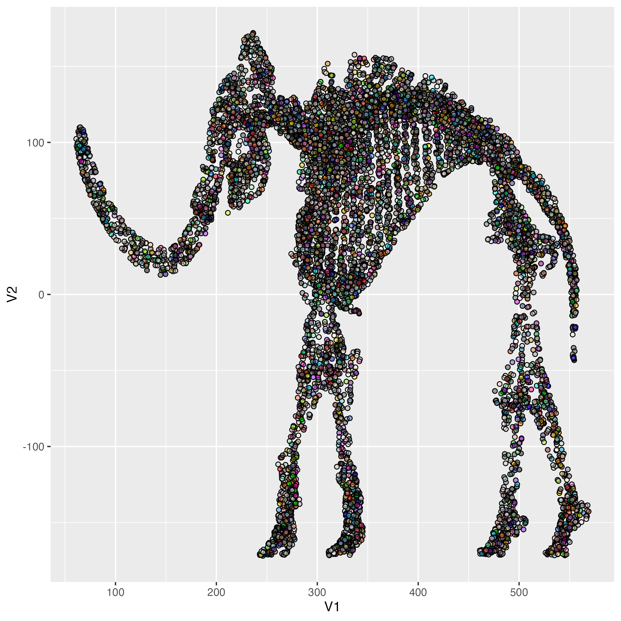
![](ggcube2_files/figure-html/my_cars_auto_08_output-1.png)
]

---
count: false

.panel1-my_cars-auto[

``` r
library(tidyverse)
library(ggcube)

ggplot(data = mammoth_df) +
  aes(x = V1) +
  aes(y = V2) +
  geom_point() +
  aes(shape = I(21)) +
  aes(fill = I(confetti)) +
* aes(color = I("white"))
```
]
 
.panel2-my_cars-auto[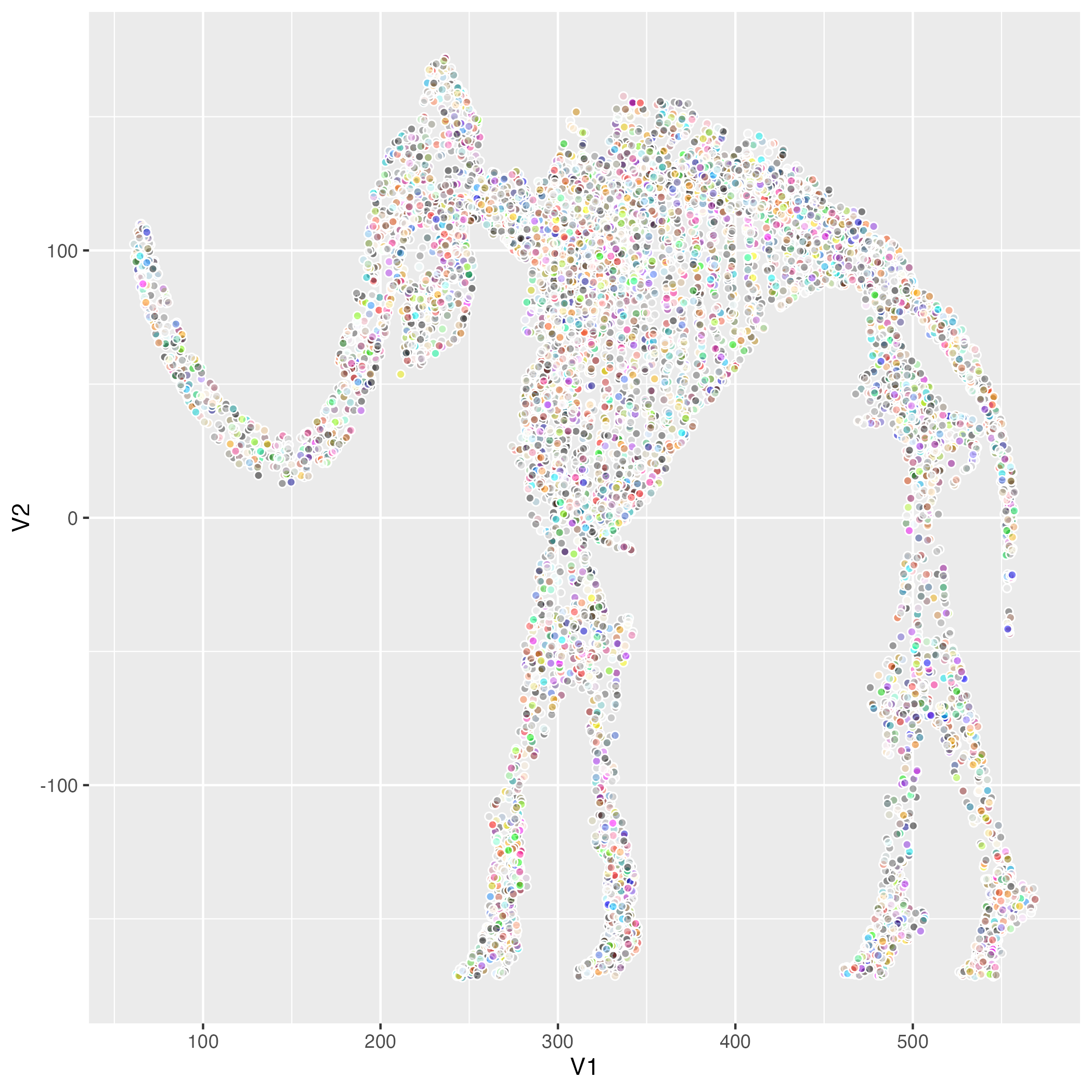
![](ggcube2_files/figure-html/my_cars_auto_09_output-1.png)
]

---
count: false

.panel1-my_cars-auto[

``` r
library(tidyverse)
library(ggcube)

ggplot(data = mammoth_df) +
  aes(x = V1) +
  aes(y = V2) +
  geom_point() +
  aes(shape = I(21)) +
  aes(fill = I(confetti)) +
  aes(color = I("white")) +
* aes(stroke = .2)
```
]
 
.panel2-my_cars-auto[
![](ggcube2_files/figure-html/my_cars_auto_10_output-1.png)
]

---
count: false

.panel1-my_cars-auto[

``` r
library(tidyverse)
library(ggcube)

ggplot(data = mammoth_df) +
  aes(x = V1) +
  aes(y = V2) +
  geom_point() +
  aes(shape = I(21)) +
  aes(fill = I(confetti)) +
  aes(color = I("white")) +
  aes(stroke = .2) +
* aes(z = V3)
```
]
 
.panel2-my_cars-auto[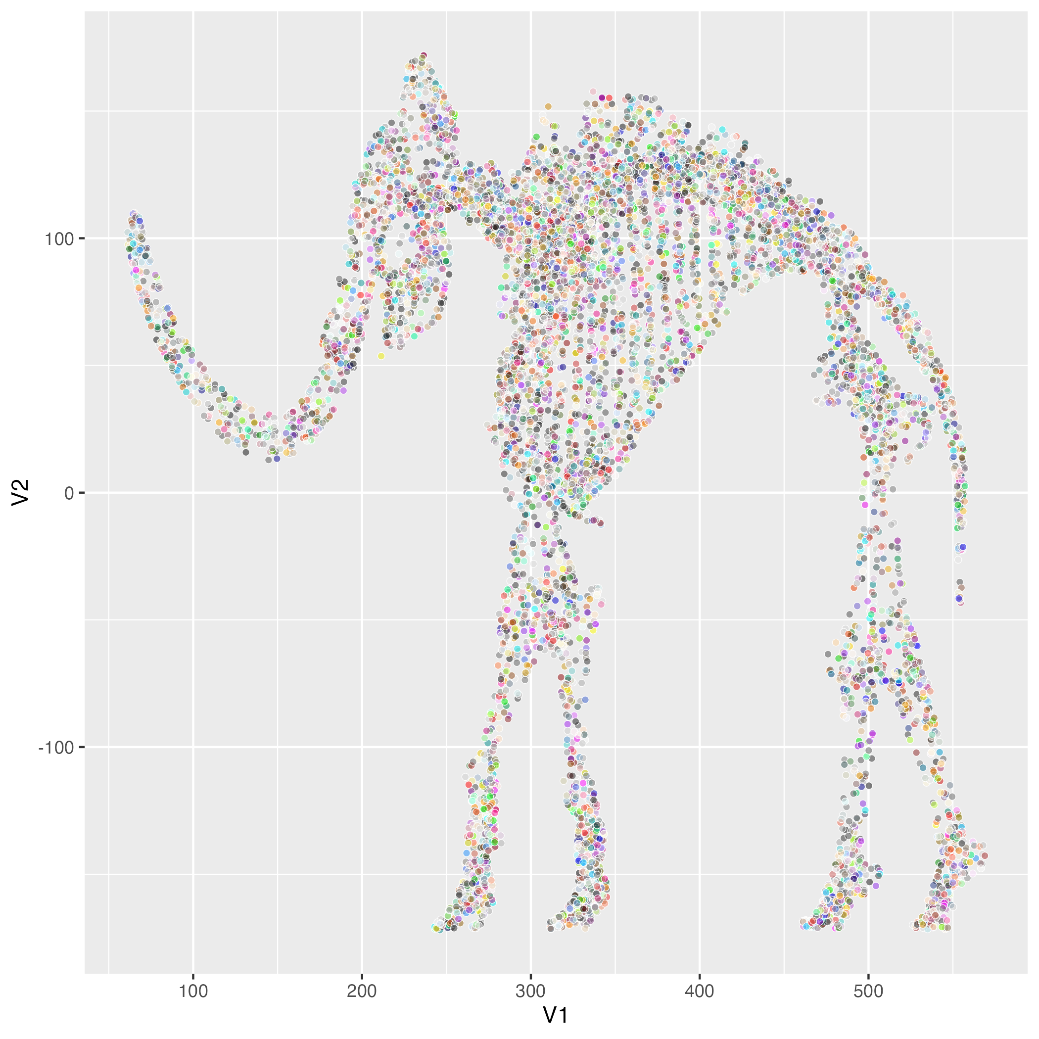
![](ggcube2_files/figure-html/my_cars_auto_11_output-1.png)
]

---
count: false

.panel1-my_cars-auto[

``` r
library(tidyverse)
library(ggcube)

ggplot(data = mammoth_df) +
  aes(x = V1) +
  aes(y = V2) +
  geom_point() +
  aes(shape = I(21)) +
  aes(fill = I(confetti)) +
  aes(color = I("white")) +
  aes(stroke = .2) +
  aes(z = V3) +
* coord_3d(ratio = c(2,1.4,1),
*          yaw = 0,
*          roll = 10,
*          pitch = 5)
```
]
 
.panel2-my_cars-auto[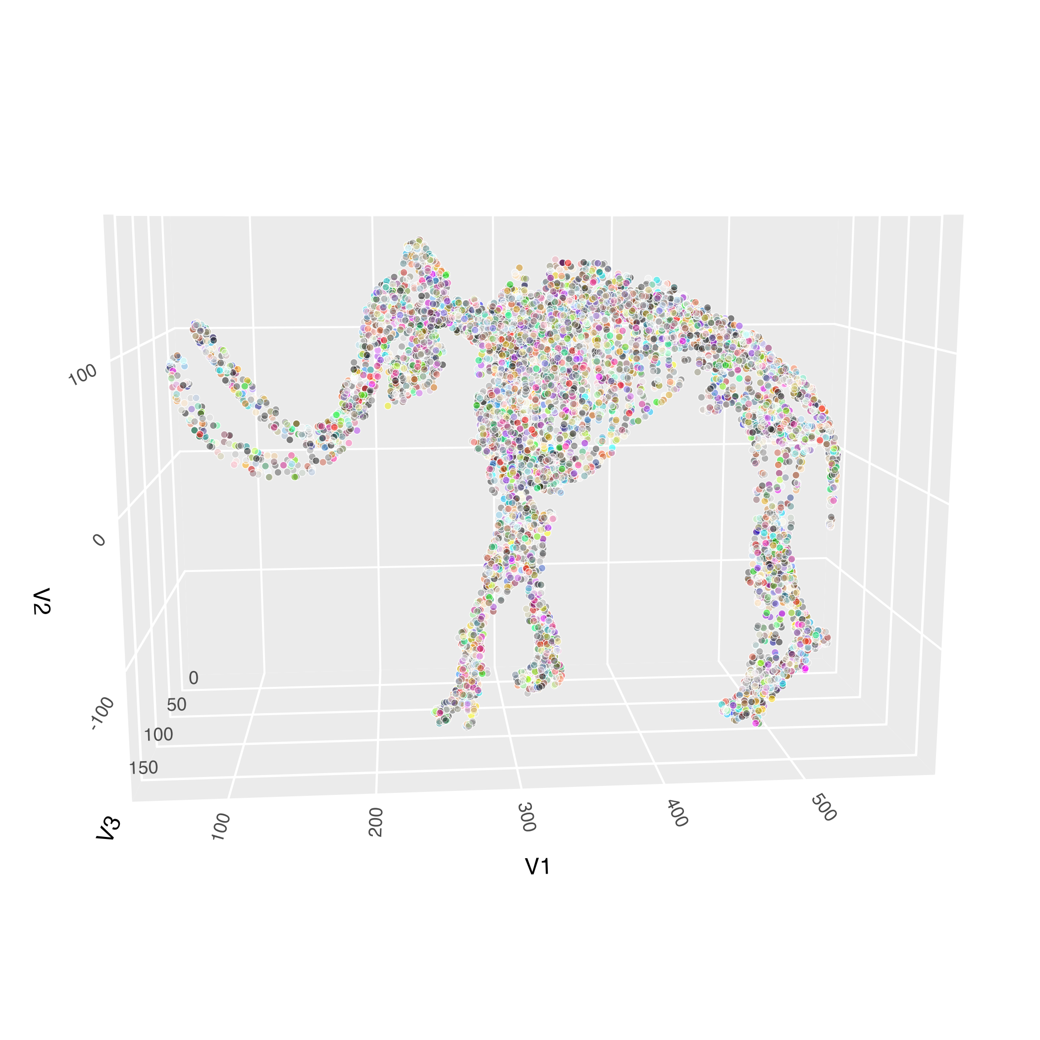
![](ggcube2_files/figure-html/my_cars_auto_12_output-1.png)
]

---
count: false

.panel1-my_cars-auto[

``` r
library(tidyverse)
library(ggcube)

ggplot(data = mammoth_df) +
  aes(x = V1) +
  aes(y = V2) +
  geom_point() +
  aes(shape = I(21)) +
  aes(fill = I(confetti)) +
  aes(color = I("white")) +
  aes(stroke = .2) +
  aes(z = V3) +
  coord_3d(ratio = c(2,1.4,1),
           yaw = 0,
           roll = 10,
           pitch = 5) +
* geom_point_3d()
```
]
 
.panel2-my_cars-auto[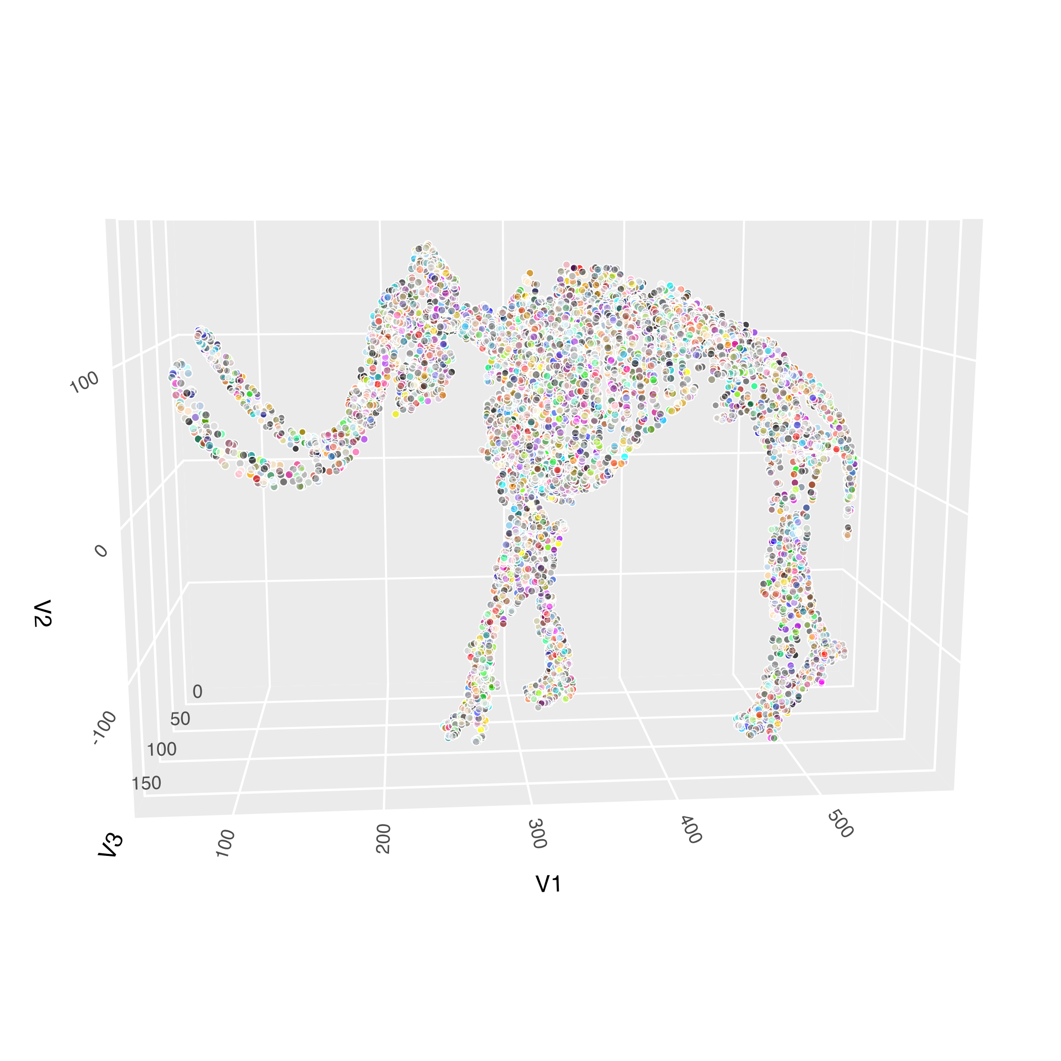
![](ggcube2_files/figure-html/my_cars_auto_13_output-1.png)
]

---
count: false

.panel1-my_cars-auto[

``` r
library(tidyverse)
library(ggcube)

ggplot(data = mammoth_df) +
  aes(x = V1) +
  aes(y = V2) +
  geom_point() +
  aes(shape = I(21)) +
  aes(fill = I(confetti)) +
  aes(color = I("white")) +
  aes(stroke = .2) +
  aes(z = V3) +
  coord_3d(ratio = c(2,1.4,1),
           yaw = 0,
           roll = 10,
           pitch = 5) +
  geom_point_3d() +
* labs(
*   title = "A Muse of ML, Max's Mammoth...",
*   subtitle = "Max Noichl popularized mammoth data, a 3D scan of a Smithsonian \nMammoth.  ML and AI researchers have turned to it in explorations like \n'Understanding UMAP' and beyond.",
*   caption = "Visualized with {ggplot2} and {ggcube} - new on CRAN!\nData as curated by Coenen and Pearce at github.com/PAIR-code/understanding-umap"
*   )
```
]
 
.panel2-my_cars-auto[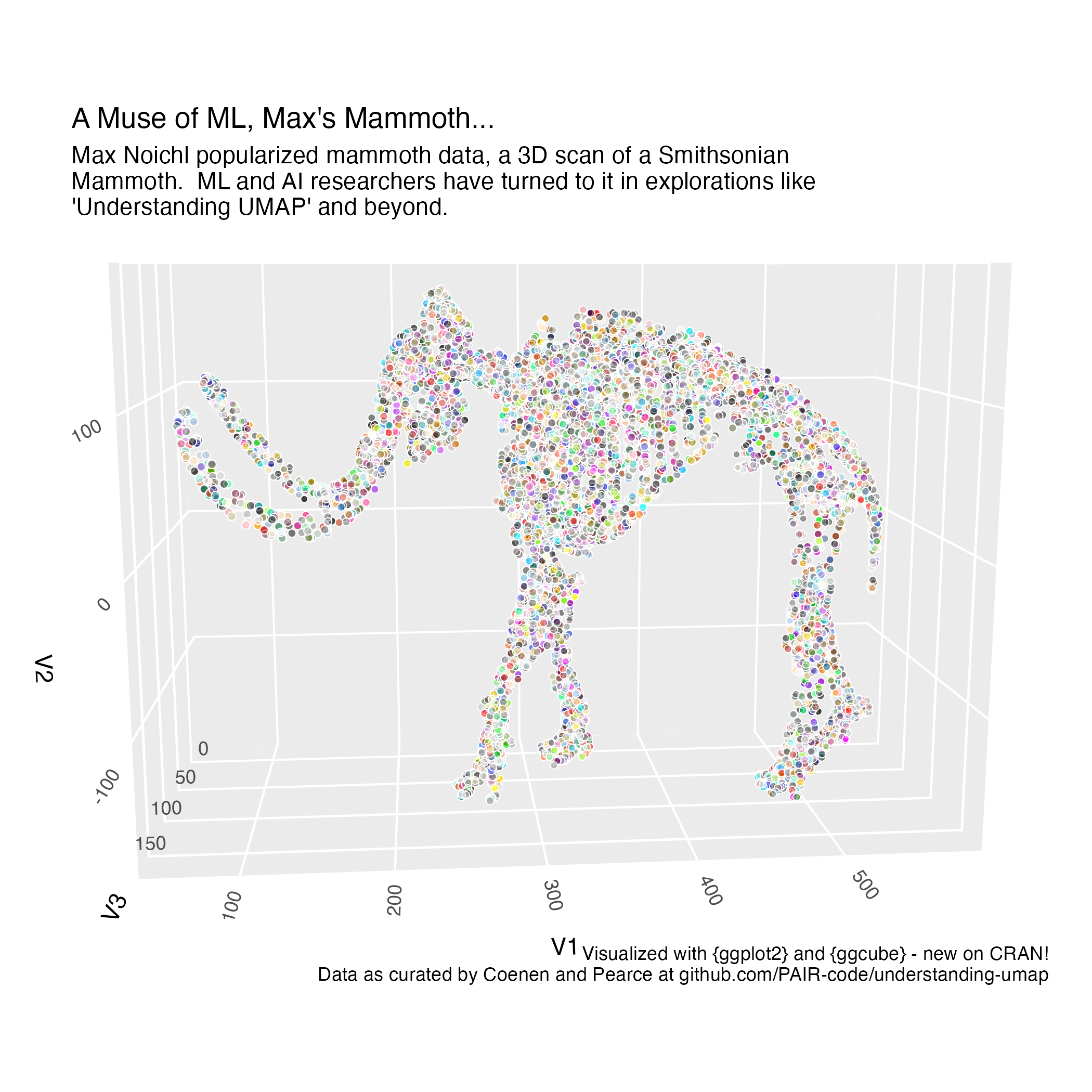
![](ggcube2_files/figure-html/my_cars_auto_14_output-1.png)
]

---
count: false

.panel1-my_cars-auto[

``` r
library(tidyverse)
library(ggcube)

ggplot(data = mammoth_df) +
  aes(x = V1) +
  aes(y = V2) +
  geom_point() +
  aes(shape = I(21)) +
  aes(fill = I(confetti)) +
  aes(color = I("white")) +
  aes(stroke = .2) +
  aes(z = V3) +
  coord_3d(ratio = c(2,1.4,1),
           yaw = 0,
           roll = 10,
           pitch = 5) +
  geom_point_3d() +
  labs(
    title = "A Muse of ML, Max's Mammoth...",
    subtitle = "Max Noichl popularized mammoth data, a 3D scan of a Smithsonian \nMammoth.  ML and AI researchers have turned to it in explorations like \n'Understanding UMAP' and beyond.",
    caption = "Visualized with {ggplot2} and {ggcube} - new on CRAN!\nData as curated by Coenen and Pearce at github.com/PAIR-code/understanding-umap"
    ) ->
* plot; animate_3d(
*   plot + theme_void(),
*   pitch = c(0, 360)
*   )
```
]
 
.panel2-my_cars-auto[
![](ggcube2_files/figure-html/my_cars_auto_15_output-1.gif)
]

<style>
.panel1-my_cars-auto {
  color: black;
  width: 38.6060606060606%;
  hight: 32%;
  float: left;
  padding-left: 1%;
  font-size: 80%
}
.panel2-my_cars-auto {
  color: black;
  width: 59.3939393939394%;
  hight: 32%;
  float: left;
  padding-left: 1%;
  font-size: 80%
}
.panel3-my_cars-auto {
  color: black;
  width: NA%;
  hight: 33%;
  float: left;
  padding-left: 1%;
  font-size: 80%
}
</style>

<style type="text/css">
.remark-code{line-height: 1.5; font-size: 80%}

@media print {
  .has-continuation {
    display: block;
  }
}

code.r.hljs.remark-code{
  position: relative;
  overflow-x: hidden;
}

code.r.hljs.remark-code:hover{
  overflow-x:visible;
  width: 500px;
  border-style: solid;
}
</style>