Simpsons’ Guest Appearances are Growing

# Simpsons’ Guest Appearances are Growing
### Adaptation of Gil Henriques’ Simpsons Plot, by Evangeline Reynolds
### 5/18/2018

---

# The original

<blockquote class="twitter-tweet"><p lang="en" dir="ltr">📈 I learned a lot doing this week&#39;s <a href="https://twitter.com/hashtag/TidyTuesday?src=hash&amp;ref_src=twsrc%5Etfw">#TidyTuesday</a>. I had to make the axes and the lines connecting the points look hand-drawn (it takes some jittering!), and learn how to put a figure in the background. Happy with the result! Code below.<a href="https://twitter.com/hashtag/dataviz?src=hash&amp;ref_src=twsrc%5Etfw">#dataviz</a> <a href="https://twitter.com/hashtag/rstats?src=hash&amp;ref_src=twsrc%5Etfw">#rstats</a> <a href="https://twitter.com/hashtag/ggplot2?src=hash&amp;ref_src=twsrc%5Etfw">#ggplot2</a> <a href="https://twitter.com/R4DScommunity?ref_src=twsrc%5Etfw">@R4DScommunity</a> <a href="https://t.co/Gr0w37pbt9">pic.twitter.com/Gr0w37pbt9</a></p>&mdash; Gil Henriques 🌹 (@_Gil_Henriques) <a href="https://twitter.com/_Gil_Henriques/status/1166373844040335360?ref_src=twsrc%5Etfw">August 27, 2019</a></blockquote> <script async src="https://platform.twitter.com/widgets.js" charset="utf-8"></script>

---

# Loading packages

```r
library(tidyverse)
```

---

# Data cleaning

---

```r
url <- "https://raw.githubusercontent.com/rfordatascience/tidytuesday/master/data/2019/2019-08-27/simpsons-guests.csv"
raw <- read_delim(file = url, delim = "|", quote = "") %>%
  mutate(number = strsplit(as.character(number), "; "))
```

---

```r
*raw
```
]]
.column[.content[

```
# A tibble: 1,386 x 6
   season number  production_code episode_title     guest_star   role      
   <chr>  <list>  <chr>           <chr>             <chr>        <chr>     
 1 1      <chr [… 7G02            Bart the Genius   Marcia Wall… Edna Krab…
 2 1      <chr [… 7G03            Homer's Odyssey   Sam McMurray Worker    
 3 1      <chr [… 7G03            Homer's Odyssey   Marcia Wall… Edna Krab…
 4 1      <chr [… 7G06            Moaning Lisa      Miriam Flynn Ms. Barr  
 5 1      <chr [… 7G06            Moaning Lisa      Ron Taylor   Bleeding …
 6 1      <chr [… 7G09            The Call of the … Albert Broo… Cowboy Bob
 7 1      <chr [… 7G07            The Telltale Head Marcia Wall… Edna Krab…
 8 1      <chr [… 7G11            Life on the Fast… Albert Broo… Jacques   
 9 1      <chr [… 7G10            Homer's Night Out Sam McMurray Gulliver …
10 1      <chr [… 7G13            The Crepes of Wr… Christian C… Gendarme …
# … with 1,376 more rows
```
]]
---
class: split-40
count: false
.column[.content[

```r
raw %>% 
* unnest()  # Splits rows that contain multiple episodes into multiple rows
```
]]
.column[.content[

```
# A tibble: 1,399 x 6
   season production_code episode_title     guest_star   role        number
   <chr>  <chr>           <chr>             <chr>        <chr>       <chr> 
 1 1      7G02            Bart the Genius   Marcia Wall… Edna Kraba… 002–1…
 2 1      7G03            Homer's Odyssey   Sam McMurray Worker      003–1…
 3 1      7G03            Homer's Odyssey   Marcia Wall… Edna Kraba… 003–1…
 4 1      7G06            Moaning Lisa      Miriam Flynn Ms. Barr    006–1…
 5 1      7G06            Moaning Lisa      Ron Taylor   Bleeding G… 006–1…
 6 1      7G09            The Call of the … Albert Broo… Cowboy Bob  007–1…
 7 1      7G07            The Telltale Head Marcia Wall… Edna Kraba… 008–1…
 8 1      7G11            Life on the Fast… Albert Broo… Jacques     009–1…
 9 1      7G10            Homer's Night Out Sam McMurray Gulliver D… 010–1…
10 1      7G13            The Crepes of Wr… Christian C… Gendarme O… 011–1…
# … with 1,389 more rows
```
]]
---
class: split-40
count: false
.column[.content[

```r
raw %>% 
  unnest() %>% # Splits rows that contain multiple episodes into multiple rows
* mutate(season = as.numeric(season))
```
]]
.column[.content[

```
# A tibble: 1,399 x 6
   season production_code episode_title     guest_star   role        number
    <dbl> <chr>           <chr>             <chr>        <chr>       <chr> 
 1      1 7G02            Bart the Genius   Marcia Wall… Edna Kraba… 002–1…
 2      1 7G03            Homer's Odyssey   Sam McMurray Worker      003–1…
 3      1 7G03            Homer's Odyssey   Marcia Wall… Edna Kraba… 003–1…
 4      1 7G06            Moaning Lisa      Miriam Flynn Ms. Barr    006–1…
 5      1 7G06            Moaning Lisa      Ron Taylor   Bleeding G… 006–1…
 6      1 7G09            The Call of the … Albert Broo… Cowboy Bob  007–1…
 7      1 7G07            The Telltale Head Marcia Wall… Edna Kraba… 008–1…
 8      1 7G11            Life on the Fast… Albert Broo… Jacques     009–1…
 9      1 7G10            Homer's Night Out Sam McMurray Gulliver D… 010–1…
10      1 7G13            The Crepes of Wr… Christian C… Gendarme O… 011–1…
# … with 1,389 more rows
```
]]
---
class: split-40
count: false
.column[.content[

```r
raw %>% 
  unnest() %>% # Splits rows that contain multiple episodes into multiple rows
  mutate(season = as.numeric(season)) %>% 
* group_by(season)
```
]]
.column[.content[

```
# A tibble: 1,399 x 6
# Groups:   season [31]
   season production_code episode_title     guest_star   role        number
    <dbl> <chr>           <chr>             <chr>        <chr>       <chr> 
 1      1 7G02            Bart the Genius   Marcia Wall… Edna Kraba… 002–1…
 2      1 7G03            Homer's Odyssey   Sam McMurray Worker      003–1…
 3      1 7G03            Homer's Odyssey   Marcia Wall… Edna Kraba… 003–1…
 4      1 7G06            Moaning Lisa      Miriam Flynn Ms. Barr    006–1…
 5      1 7G06            Moaning Lisa      Ron Taylor   Bleeding G… 006–1…
 6      1 7G09            The Call of the … Albert Broo… Cowboy Bob  007–1…
 7      1 7G07            The Telltale Head Marcia Wall… Edna Kraba… 008–1…
 8      1 7G11            Life on the Fast… Albert Broo… Jacques     009–1…
 9      1 7G10            Homer's Night Out Sam McMurray Gulliver D… 010–1…
10      1 7G13            The Crepes of Wr… Christian C… Gendarme O… 011–1…
# … with 1,389 more rows
```
]]
---
class: split-40
count: false
.column[.content[

```r
raw %>% 
  unnest() %>% # Splits rows that contain multiple episodes into multiple rows
  mutate(season = as.numeric(season)) %>% 
  group_by(season) %>% 
* summarize(guests_per_episode =
*             n_distinct(guest_star) /
*             n_distinct(number))
```
]]
.column[.content[

```
# A tibble: 31 x 2
   season guests_per_episode
    <dbl>              <dbl>
 1      1               1   
 2      2               1.47
 3      3               1.57
 4      4               1.37
 5      5               1.47
 6      6               1.45
 7      7               1.32
 8      8               1.53
 9      9               1.48
10     10               2.35
# … with 21 more rows
```
]]
---
class: split-40
count: false
.column[.content[

```r
raw %>% 
  unnest() %>% # Splits rows that contain multiple episodes into multiple rows
  mutate(season = as.numeric(season)) %>% 
  group_by(season) %>% 
  summarize(guests_per_episode = 
              n_distinct(guest_star) / 
              n_distinct(number)) -> 
*clean_data
```
]]
.column[.content[

]]

---

# Attention to detail:  "Hand drawing"

One thing that is so charming about this plot is the feeling that Bart Simpson has hand-drawn the figure.

Gil writes: *I want the axes and the line connecting the points to look hand-drawn, so I will use geom_line + jitter to draw them*

---

# spline() to connect points

He uses the spline function, which makes a smooth connection between points, rather than sharp, as a human might do in a rush.

Here is the function:

spline(x, y = NULL, n = 3*length(x), method = "fmm",
       xmin = min(x), xmax = max(x), xout, ties = mean)

And the description:

"Perform cubic (or Hermite) [spline interpolation](https://en.wikipedia.org/wiki/Spline_interpolation) of given data points, returning either a list of points obtained by the interpolation or a function performing the interpolation."

---

```r
*as.data.frame(spline(x = clean_data$season,
*                    y = clean_data$guests_per_episode,
*                    method = "natural"))
```
]]
.column[.content[

```
           x        y
1   1.000000 1.000000
2   1.325843 1.174043
3   1.651685 1.333329
4   1.977528 1.463101
5   2.303371 1.550189
6   2.629213 1.589227
7   2.955056 1.577250
8   3.280899 1.515911
9   3.606742 1.434941
10  3.932584 1.374621
11  4.258427 1.369256
12  4.584270 1.407839
13  4.910112 1.458662
14  5.235955 1.491804
15  5.561798 1.495347
16  5.887640 1.467322
17  6.213483 1.407902
18  6.539326 1.342004
19  6.865169 1.310998
20  7.191011 1.352768
21  7.516854 1.445296
22  7.842697 1.518755
23  8.168539 1.506376
24  8.494382 1.434654
25  8.820225 1.419246
26  9.146067 1.575162
27  9.471910 1.892077
28  9.797753 2.216208
29 10.123596 2.388315
30 10.449438 2.355107
31 10.775281 2.208644
32 11.101124 2.050824
33 11.426966 1.934197
34 11.752809 1.829967
35 12.078652 1.702036
36 12.404494 1.553335
37 12.730337 1.464417
38 13.056180 1.524809
39 13.382022 1.760170
40 13.707865 2.042141
41 14.033708 2.219656
42 14.359551 2.198243
43 14.685393 2.049906
44 15.011236 1.877104
45 15.337079 1.764001
46 15.662921 1.728769
47 15.988764 1.774706
48 16.314607 1.896317
49 16.640449 2.049109
50 16.966292 2.177779
51 17.292135 2.238360
52 17.617978 2.248857
53 17.943820 2.248341
54 18.269663 2.265795
55 18.595506 2.261781
56 18.921348 2.168493
57 19.247191 1.932390
58 19.573034 1.621352
59 19.898876 1.364317
60 20.224719 1.280641
61 20.550562 1.382170
62 20.876404 1.615532
63 21.202247 1.924794
64 21.528090 2.231301
65 21.853933 2.439836
66 22.179775 2.461947
67 22.505618 2.339465
68 22.831461 2.228049
69 23.157303 2.280524
70 23.483146 2.483319
71 23.808989 2.648812
72 24.134831 2.586330
73 24.460674 2.289811
74 24.786517 1.984472
75 25.112360 1.906898
76 25.438202 2.113560
77 25.764045 2.390166
78 26.089888 2.501732
79 26.415730 2.368742
80 26.741573 2.193013
81 27.067416 2.205279
82 27.393258 2.498667
83 27.719101 2.865166
84 28.044944 3.057107
85 28.370787 2.935942
86 28.696629 2.653548
87 29.022472 2.409573
88 29.348315 2.348194
89 29.674157 2.433004
90 30.000000 2.590909
```
]]
---
class: split-40
count: false
.column[.content[

```r
as.data.frame(spline(x = clean_data$season, 
                     y = clean_data$guests_per_episode, 
                     method = "natural")) -> 
* spline_int
```
]]
.column[.content[

]]

---

# "Hand drawn" axes with position_jitter()

Then Gil also creates mini datasets for hand drawn axes x and y.  He creates straight horizontal and vertical lines, segmented into small pieces.  He plots these mini data sets with geom_line where the position is jittered.

---

```r
*data.frame(x = seq(from = 0, to = 30, by = 1),
*          y = rep(0, 31))
```
]]
.column[.content[

```
    x y
1   0 0
2   1 0
3   2 0
4   3 0
5   4 0
6   5 0
7   6 0
8   7 0
9   8 0
10  9 0
11 10 0
12 11 0
13 12 0
14 13 0
15 14 0
16 15 0
17 16 0
18 17 0
19 18 0
20 19 0
21 20 0
22 21 0
23 22 0
24 23 0
25 24 0
26 25 0
27 26 0
28 27 0
29 28 0
30 29 0
31 30 0
```
]]
---
class: split-40
count: false
.column[.content[

```r
data.frame(x = seq(from = 0, to = 30, by = 1), 
           y = rep(0, 31)) -> 
* drawn.x.axis
```
]]
.column[.content[

]]
---
class: split-40
count: false
.column[.content[

```r
data.frame(x = seq(from = 0, to = 30, by = 1), 
           y = rep(0, 31)) -> 
  drawn.x.axis 
*data.frame(x = rep(0, 21),
*          y = seq(from = 0, to = 4, by = 0.2))
```
]]
.column[.content[

```
   x   y
1  0 0.0
2  0 0.2
3  0 0.4
4  0 0.6
5  0 0.8
6  0 1.0
7  0 1.2
8  0 1.4
9  0 1.6
10 0 1.8
11 0 2.0
12 0 2.2
13 0 2.4
14 0 2.6
15 0 2.8
16 0 3.0
17 0 3.2
18 0 3.4
19 0 3.6
20 0 3.8
21 0 4.0
```
]]
---
class: split-40
count: false
.column[.content[

```r
data.frame(x = seq(from = 0, to = 30, by = 1), 
           y = rep(0, 31)) -> 
  drawn.x.axis 
data.frame(x = rep(0, 21), 
           y = seq(from = 0, to = 4, by = 0.2)) -> 
* drawn.y.axis
```
]]
.column[.content[

]]

---
# Plotting

---

```r
*clean_data
```
]]
.column[.content[

```r
clean_data %>% 
* ggplot()
```
]]
.column[.content[
![](simpsons_files/figure-html/output_plotting_2-1.png)
]]
---
class: split-40
count: false
.column[.content[

```r
clean_data %>% 
  ggplot() + 
* aes(x = season)
```
]]
.column[.content[
![](simpsons_files/figure-html/output_plotting_3-1.png)
]]
---
class: split-40
count: false
.column[.content[

```r
clean_data %>% 
  ggplot() + 
  aes(x = season) + 
* aes(y = guests_per_episode)
```
]]
.column[.content[
![](simpsons_files/figure-html/output_plotting_4-1.png)
]]
---
class: split-40
count: false
.column[.content[

```r
clean_data %>% 
  ggplot() + 
  aes(x = season) + 
  aes(y = guests_per_episode) + 
* geom_point(size = 4, color = "snow3")
```
]]
.column[.content[
![](simpsons_files/figure-html/output_plotting_5-1.png)
]]
---
class: split-40
count: false
.column[.content[

```r
clean_data %>% 
  ggplot() + 
  aes(x = season) + 
  aes(y = guests_per_episode) + 
  geom_point(size = 4, color = "snow3") + 
* geom_line(data = spline_int,
*           mapping = aes(x = x, y = y),
*           color = "snow3", size = 0.8,
*           position = position_jitter(w = 0.05, h = 0.05))
```
]]
.column[.content[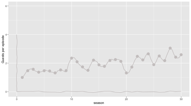
![](simpsons_files/figure-html/output_plotting_9-1.png)
]]
---
class: split-40
count: false
.column[.content[

```r
clean_data %>% 
  ggplot() + 
  aes(x = season) + 
  aes(y = guests_per_episode) + 
  geom_point(size = 4, color = "snow3") + 
  geom_line(data = spline_int, 
            mapping = aes(x = x, y = y), 
            color = "snow3", size = 0.8, 
            position = position_jitter(w = 0.05, h = 0.05)) + 
  geom_line(data = drawn.x.axis, 
            mapping = aes(x = x, y = y), 
            color = "snow3", size = 0.8, 
            position = position_jitter(w = 0.0, h = 0.05)) + 
  geom_line(data = drawn.y.axis, 
            mapping = aes(x = x, y = y), 
            color = "snow3", size = 0.8, 
            position = position_jitter(w = 0.05, h = 0.0)) + 
  labs(y = "Guests per episode") + 
  labs(x = "Season") + 
  labs(title = "The number of guest stars in\nthe Simpsons is increasing") + 
  labs(caption = "@_Gil_Henriques for #TidyTuesday") + 
  ylim(-0.1, 4.3) + 
  xlim(-0.1, 30.5) + 
  theme_void() + 
* theme(axis.text = element_text(size = 15,
*                                  color = "snow3"))
```
]]
.column[.content[
![](simpsons_files/figure-html/output_plotting_26-1.png)
]]
---
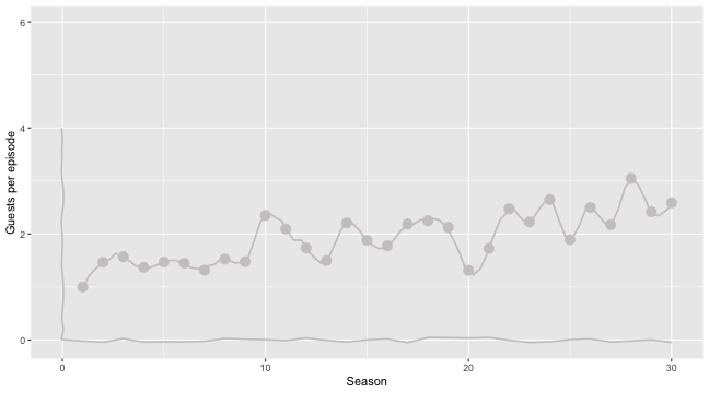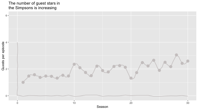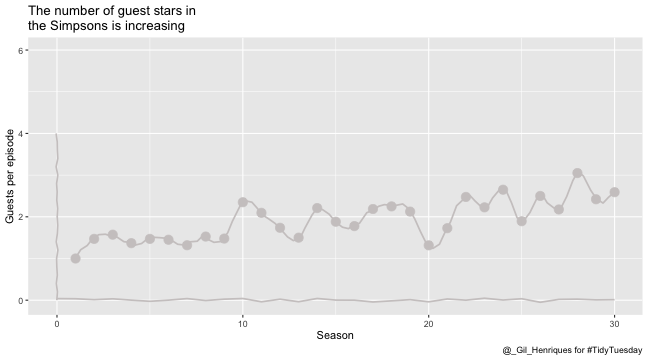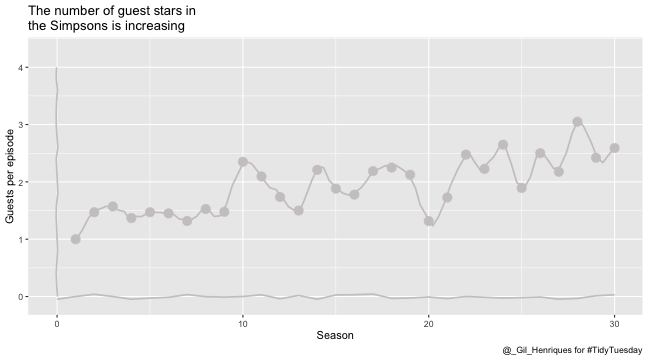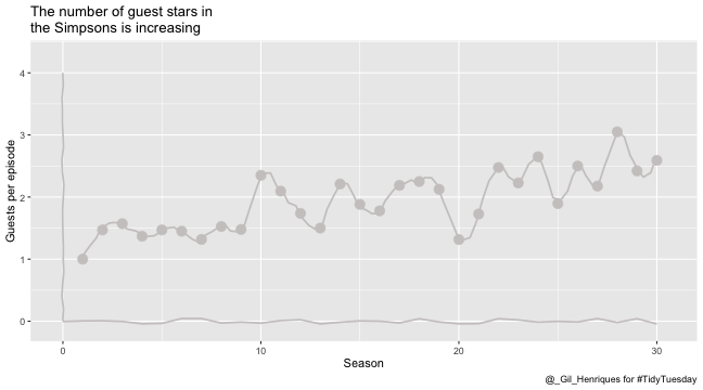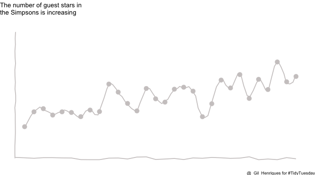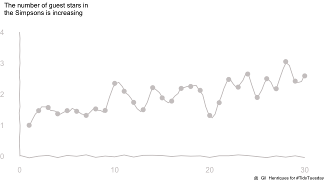class: split-40
count: false
.column[.content[

```r
clean_data %>% 
  ggplot() + 
  aes(x = season) + 
  aes(y = guests_per_episode) + 
  geom_point(size = 4, color = "snow3") + 
  geom_line(data = spline_int, 
            mapping = aes(x = x, y = y), 
            color = "snow3", size = 0.8, 
            position = position_jitter(w = 0.05, h = 0.05)) + 
  geom_line(data = drawn.x.axis, 
            mapping = aes(x = x, y = y), 
            color = "snow3", size = 0.8, 
            position = position_jitter(w = 0.0, h = 0.05)) + 
  geom_line(data = drawn.y.axis, 
            mapping = aes(x = x, y = y), 
            color = "snow3", size = 0.8, 
            position = position_jitter(w = 0.05, h = 0.0)) + 
  labs(y = "Guests per episode") + 
  labs(x = "Season") + 
  labs(title = "The number of guest stars in\nthe Simpsons is increasing") + 
  labs(caption = "@_Gil_Henriques for #TidyTuesday") + 
  ylim(-0.1, 4.3) + 
  xlim(-0.1, 30.5) + 
  theme_void() + 
  theme(axis.text = element_text(size = 15, 
                                   color = "snow3")) + 
* theme(axis.title = element_text(size = 20, color = "snow3"))
```
]]
.column[.content[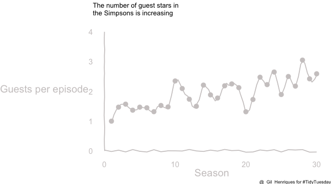
![](simpsons_files/figure-html/output_plotting_27-1.png)
]]
---
class: split-40
count: false
.column[.content[

```r
clean_data %>% 
  ggplot() + 
  aes(x = season) + 
  aes(y = guests_per_episode) + 
  geom_point(size = 4, color = "snow3") + 
  geom_line(data = spline_int, 
            mapping = aes(x = x, y = y), 
            color = "snow3", size = 0.8, 
            position = position_jitter(w = 0.05, h = 0.05)) + 
  geom_line(data = drawn.x.axis, 
            mapping = aes(x = x, y = y), 
            color = "snow3", size = 0.8, 
            position = position_jitter(w = 0.0, h = 0.05)) + 
  geom_line(data = drawn.y.axis, 
            mapping = aes(x = x, y = y), 
            color = "snow3", size = 0.8, 
            position = position_jitter(w = 0.05, h = 0.0)) + 
  labs(y = "Guests per episode") + 
  labs(x = "Season") + 
  labs(title = "The number of guest stars in\nthe Simpsons is increasing") + 
  labs(caption = "@_Gil_Henriques for #TidyTuesday") + 
  ylim(-0.1, 4.3) + 
  xlim(-0.1, 30.5) + 
  theme_void() + 
  theme(axis.text = element_text(size = 15, 
                                   color = "snow3")) + 
  theme(axis.title = element_text(size = 20, color = "snow3")) + 
* theme(plot.title = element_text(size = 25, face = "bold",
*                                 color = "snow3",
*                                 hjust = 0.5))
```
]]
.column[.content[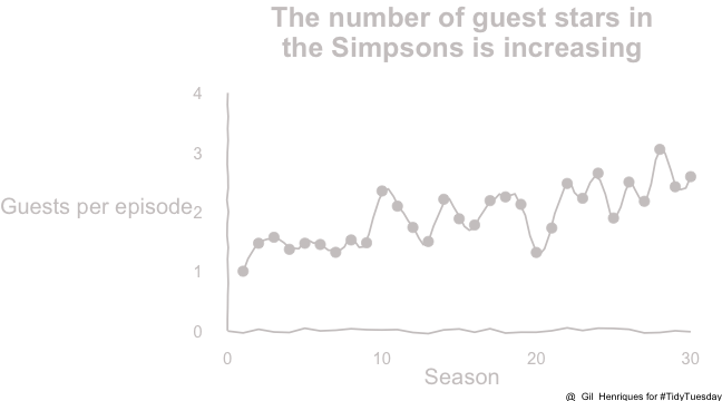
![](simpsons_files/figure-html/output_plotting_30-1.png)
]]
---
class: split-40
count: false
.column[.content[

```r
clean_data %>% 
  ggplot() + 
  aes(x = season) + 
  aes(y = guests_per_episode) + 
  geom_point(size = 4, color = "snow3") + 
  geom_line(data = spline_int, 
            mapping = aes(x = x, y = y), 
            color = "snow3", size = 0.8, 
            position = position_jitter(w = 0.05, h = 0.05)) + 
  geom_line(data = drawn.x.axis, 
            mapping = aes(x = x, y = y), 
            color = "snow3", size = 0.8, 
            position = position_jitter(w = 0.0, h = 0.05)) + 
  geom_line(data = drawn.y.axis, 
            mapping = aes(x = x, y = y), 
            color = "snow3", size = 0.8, 
            position = position_jitter(w = 0.05, h = 0.0)) + 
  labs(y = "Guests per episode") + 
  labs(x = "Season") + 
  labs(title = "The number of guest stars in\nthe Simpsons is increasing") + 
  labs(caption = "@_Gil_Henriques for #TidyTuesday") + 
  ylim(-0.1, 4.3) + 
  xlim(-0.1, 30.5) + 
  theme_void() + 
  theme(axis.text = element_text(size = 15, 
                                   color = "snow3")) + 
  theme(axis.title = element_text(size = 20, color = "snow3")) + 
  theme(plot.title = element_text(size = 25, face = "bold", 
                                  color = "snow3", 
                                  hjust = 0.5)) + 
* theme(plot.caption = element_text(color = "snow3"))
```
]]
.column[.content[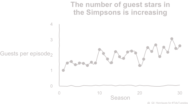
![](simpsons_files/figure-html/output_plotting_31-1.png)
]]
---
class: split-40
count: false
.column[.content[

```r
clean_data %>% 
  ggplot() + 
  aes(x = season) + 
  aes(y = guests_per_episode) + 
  geom_point(size = 4, color = "snow3") + 
  geom_line(data = spline_int, 
            mapping = aes(x = x, y = y), 
            color = "snow3", size = 0.8, 
            position = position_jitter(w = 0.05, h = 0.05)) + 
  geom_line(data = drawn.x.axis, 
            mapping = aes(x = x, y = y), 
            color = "snow3", size = 0.8, 
            position = position_jitter(w = 0.0, h = 0.05)) + 
  geom_line(data = drawn.y.axis, 
            mapping = aes(x = x, y = y), 
            color = "snow3", size = 0.8, 
            position = position_jitter(w = 0.05, h = 0.0)) + 
  labs(y = "Guests per episode") + 
  labs(x = "Season") + 
  labs(title = "The number of guest stars in\nthe Simpsons is increasing") + 
  labs(caption = "@_Gil_Henriques for #TidyTuesday") + 
  ylim(-0.1, 4.3) + 
  xlim(-0.1, 30.5) + 
  theme_void() + 
  theme(axis.text = element_text(size = 15, 
                                   color = "snow3")) + 
  theme(axis.title = element_text(size = 20, color = "snow3")) + 
  theme(plot.title = element_text(size = 25, face = "bold", 
                                  color = "snow3", 
                                  hjust = 0.5)) + 
  theme(plot.caption = element_text(color = "snow3")) + 
* theme(plot.margin = margin(t = 1, r = 3, b = 1, l = 1, "cm"))
```
]]
.column[.content[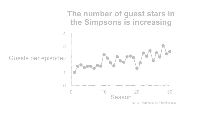
![](simpsons_files/figure-html/output_plotting_32-1.png)
]]
---
class: split-40
count: false
.column[.content[

```r
clean_data %>% 
  ggplot() + 
  aes(x = season) + 
  aes(y = guests_per_episode) + 
  geom_point(size = 4, color = "snow3") + 
  geom_line(data = spline_int, 
            mapping = aes(x = x, y = y), 
            color = "snow3", size = 0.8, 
            position = position_jitter(w = 0.05, h = 0.05)) + 
  geom_line(data = drawn.x.axis, 
            mapping = aes(x = x, y = y), 
            color = "snow3", size = 0.8, 
            position = position_jitter(w = 0.0, h = 0.05)) + 
  geom_line(data = drawn.y.axis, 
            mapping = aes(x = x, y = y), 
            color = "snow3", size = 0.8, 
            position = position_jitter(w = 0.05, h = 0.0)) + 
  labs(y = "Guests per episode") + 
  labs(x = "Season") + 
  labs(title = "The number of guest stars in\nthe Simpsons is increasing") + 
  labs(caption = "@_Gil_Henriques for #TidyTuesday") + 
  ylim(-0.1, 4.3) + 
  xlim(-0.1, 30.5) + 
  theme_void() + 
  theme(axis.text = element_text(size = 15, 
                                   color = "snow3")) + 
  theme(axis.title = element_text(size = 20, color = "snow3")) + 
  theme(plot.title = element_text(size = 25, face = "bold", 
                                  color = "snow3", 
                                  hjust = 0.5)) + 
  theme(plot.caption = element_text(color = "snow3")) + 
  theme(plot.margin = margin(t = 1, r = 3, b = 1, l = 1, "cm"))  + 
* theme(axis.title.y = element_text(angle = 90))
```
]]
.column[.content[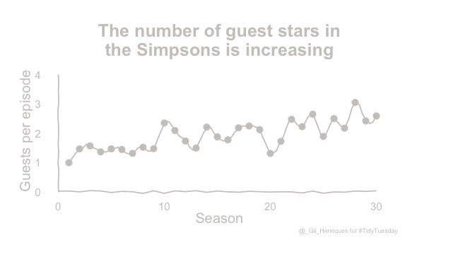
![](simpsons_files/figure-html/output_plotting_33-1.png)
]]
---
class: split-40
count: false
.column[.content[

```r
clean_data %>% 
  ggplot() + 
  aes(x = season) + 
  aes(y = guests_per_episode) + 
  geom_point(size = 4, color = "snow3") + 
  geom_line(data = spline_int, 
            mapping = aes(x = x, y = y), 
            color = "snow3", size = 0.8, 
            position = position_jitter(w = 0.05, h = 0.05)) + 
  geom_line(data = drawn.x.axis, 
            mapping = aes(x = x, y = y), 
            color = "snow3", size = 0.8, 
            position = position_jitter(w = 0.0, h = 0.05)) + 
  geom_line(data = drawn.y.axis, 
            mapping = aes(x = x, y = y), 
            color = "snow3", size = 0.8, 
            position = position_jitter(w = 0.05, h = 0.0)) + 
  labs(y = "Guests per episode") + 
  labs(x = "Season") + 
  labs(title = "The number of guest stars in\nthe Simpsons is increasing") + 
  labs(caption = "@_Gil_Henriques for #TidyTuesday") + 
  ylim(-0.1, 4.3) + 
  xlim(-0.1, 30.5) + 
  theme_void() + 
  theme(axis.text = element_text(size = 15, 
                                   color = "snow3")) + 
  theme(axis.title = element_text(size = 20, color = "snow3")) + 
  theme(plot.title = element_text(size = 25, face = "bold", 
                                  color = "snow3", 
                                  hjust = 0.5)) + 
  theme(plot.caption = element_text(color = "snow3")) + 
  theme(plot.margin = margin(t = 1, r = 3, b = 1, l = 1, "cm"))  + 
  theme(axis.title.y = element_text(angle = 90)) -> 
*plot
```
]]
.column[.content[

]]

---

# Adding background

---

```r
*simpsons_gif_url <- "https://github.com/GilHenriques/TidyTuesdays/blob/master/2019-08-27%20Simpsons%20guest%20stars/chalkboard_simpsons.gif?raw=true"
```
]]
.column[.content[

]]
---
class: split-40
count: false
.column[.content[

```r
simpsons_gif_url <- "https://github.com/GilHenriques/TidyTuesdays/blob/master/2019-08-27%20Simpsons%20guest%20stars/chalkboard_simpsons.gif?raw=true" 
*plot
```
]]
.column[.content[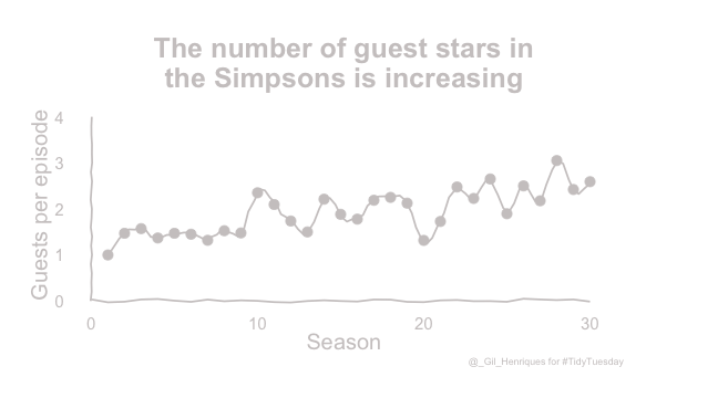
![](simpsons_files/figure-html/output_simpsons_2-1.png)
]]
---
class: split-40
count: false
.column[.content[

```r
simpsons_gif_url <- "https://github.com/GilHenriques/TidyTuesdays/blob/master/2019-08-27%20Simpsons%20guest%20stars/chalkboard_simpsons.gif?raw=true" 
plot %>% 
* ggimage::ggbackground(
*   background = simpsons_gif_url,
*   by = "height")
```
]]
.column[.content[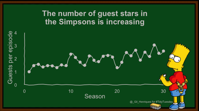
![](simpsons_files/figure-html/output_simpsons_5-1.png)
]]

---

# Changes from the [original](https://github.com/GilHenriques/TidyTuesdays) and notes to self

- I use [slow ggplot principles](https://evamaerey.github.io/ggplot_flipbook/ggplot_flipbook_xaringan.html#3) to provide maximal feedback for each step of the build. 
- Fonts are still tricky to manage across platforms and in the flipbook setting, so sadly I don't do anything with them, and a less charming plot results.
- I changed the text color to be off white instead of white, so that you can see it against the theme_void() white background
- There seems to be some problem with the display when there are list columns in data relates to square brackets. hmmmmm...
- This should be included in [TidyTuesday walk-throughs](https://evamaerey.github.io/tidytuesday_walk_through/tidytuesday_highlights.html#1) at some point.

---