- ggcalendar
- Step 00. Convenience functions, dates vectors to data frames.
- Step 1 & 2. Compute: from date to x/y, & define StatCalendar
-
Step 3. Let’s write a user-facing function
stat_calendar() - aliasing and convenience
-
defaults_calendar&ggcalendar()Thinking about set of scales/coords etc, that gives you a nice calendar (to wrap up into defaults) - NYC flights Example
- Births example
- data defaults to calendar year and aes(date = date)
- Minimal Viable Packaging
- Traditional README
- more ideas
Note: This README walks through package rational and contains the code that defines proposed package functions and in addition to first-cut testing. TLDR - Jump to traditional readme content
Here’s a proposal for creating calendars with ggplot2 via Stat extension.
When using calendars, ‘when?’ and ‘where?’ are the same question! So, ggcalendar introduces a new positional aesthetic: ‘date’. Let’s put things on the calendar!
In this proposed package, we’ll specify the position of a calendar event calendar using dates as the required aesthetic: aes(date = my_variable_of_dates)! Then you can use layers function stat_calendar() and derivative geom functions geom_text_calendar, geom_tile_calendar and geom_point_calendar to place specific grobs/mark in the plot space.
Under the hood, the compute_group functions finds the x and y position for the date in the month (x is day in week and y is week in month). Faceting by month is used to prevent over-plotting.
Other possible directions would be to calculate x and y based on date in month and on month - instead of relying on faceting by month. Furthermore, a dedicated Coord could be created (Teun’s thought). Then maybe dates would just feed generically in as the ‘x’ aes - this sounds cool!
# install.packages("devtools")
devtools::install_github("EvaMaeRey/ggcalendar")
Step 00. Convenience functions, dates vectors to data frames.
Because ggplot2’s diet is consists solely of dataframes, we create a number of convenience functions that will help us produce dataframes with column ‘date’ we can feed into ggplot2.
knitrExtra:::chunk_to_r("df")
df_today <- function(){

  data.frame(date = Sys.Date())

}

df_day <- function(date = NULL){

  if(is.null(date)){date <- Sys.Date()}

  data.frame(date = date)

}


df_dates_interval <- function(start_date, end_date){

  data.frame(date = as.Date(start_date):as.Date(end_date) |>
    as.Date())

}

df_month <- function(month = NULL, year = NULL){

  if(is.null(month)){

    date <- Sys.Date()
    month <- lubridate::month(date)
  }

  if(is.numeric(month)){

    month <- stringr::str_pad(month, width = 2, pad = "0")

  }

    if(is.null(year)){

    date <- Sys.Date()
    year <- lubridate::year(date)
    }


  paste0(year,"-", month, "-01") |>
    lubridate::as_date() ->
    start_date

  start_date |> lubridate::ceiling_date(unit = "month") ->
    end_date

    data.frame(date =
                 df_dates_interval(start_date,
                                       end_date - lubridate::days(1)))

}

df_week <- function(date = NULL){

  if(is.null(date)){date <- Sys.Date()}

  start_date <- lubridate::floor_date(date, unit = "week")
  end_date <- lubridate::ceiling_date(date, unit = "week")

  data.frame(date = df_dates_interval(start_date,
                        end_date - lubridate::days(1)) )

}

return_df_hours_week <- function(date = NULL){

  if(is.null(date)){date <- Sys.Date()}

  start_date <- lubridate::floor_date(date, unit = "week")

  data.frame(date = (start_date + lubridate::hours(1:(24*7-1))))

}

df_year <- function(year = NULL){

  if(is.null(year)){year <-  lubridate::year(Sys.Date())}

  paste0(year, "-01-01") |>
    lubridate::as_date() ->
  start_date

  start_date |> lubridate::ceiling_date(unit = "year") ->
    end_date

    data.frame(date =
                 df_dates_interval(start_date,
                                       end_date - lubridate::days(1)))

}
Examples
Let’s have a look at some of these.
df_today()
#>         date
#> 1 2024-05-16

df_day()
#>         date
#> 1 2024-05-16

df_dates_interval(start_date = "2024-10-02", end_date = "2024-10-04")
#>         date
#> 1 2024-10-02
#> 2 2024-10-03
#> 3 2024-10-04

df_week()
#>         date
#> 1 2024-05-12
#> 2 2024-05-13
#> 3 2024-05-14
#> 4 2024-05-15
#> 5 2024-05-16
#> 6 2024-05-17
#> 7 2024-05-18

df_year() |> head()
#>         date
#> 1 2024-01-01
#> 2 2024-01-02
#> 3 2024-01-03
#> 4 2024-01-04
#> 5 2024-01-05
#> 6 2024-01-06

df_month() |> head()
#>         date
#> 1 2024-05-01
#> 2 2024-05-02
#> 3 2024-05-03
#> 4 2024-05-04
#> 5 2024-05-05
#> 6 2024-05-06

return_df_hours_week() |> head()
#>                  date
#> 1 2024-05-12 01:00:00
#> 2 2024-05-12 02:00:00
#> 3 2024-05-12 03:00:00
#> 4 2024-05-12 04:00:00
#> 5 2024-05-12 05:00:00
#> 6 2024-05-12 06:00:00
Step 1 & 2. Compute: from date to x/y, & define StatCalendar
The computation that we want to be done under the hood relates to translating the here-to-fore unknown positional aesthetic ‘date’ to the first-class ‘x’ and ‘y’ positional aesthetic mappings, as well as variables that can be used in faceting (month).
knitrExtra:::chunk_to_r("get_week_of_month")As a pre-step to computing many useful variables from our date variable, we focus on this (currently messy) conversion of vectors of dates to week of the month.
get_week_of_month <- function(x){

  (- lubridate::wday(x) + lubridate::day(x)) %/%
    7 + 1 +
    ifelse(lubridate::wday(lubridate::floor_date(lubridate::as_date(x), "month")) == 1, 0, 1)

}
Next, we’ll define a compute group function. A number of variables are created by parsing our date variable.
Then, we’ll pass all this computation to define a new ggproto object StatCalendar. For maximum flexibility, our compute function doesn’t create ggplot2 core aesthetic channels ‘x’, ‘y’, and ‘label’ variables, but instead uses the default_aes field to state what should be first interpreted as x, y and label (thoughts? Maybe only ‘label’ should be managed like this).
knitrExtra:::chunk_to_r("compute_group_calendar")
compute_group_calendar <- function(data, scales){

  data |>
    dplyr::mutate(wday = lubridate::wday(.data$date)) |>
    dplyr::mutate(wday_abbr = lubridate::wday(.data$date, label = TRUE, abbr = TRUE)) |>
    dplyr::mutate(week_of_month = get_week_of_month(.data$date)) |>
    dplyr::mutate(day = lubridate::day(.data$date)) |>
    dplyr::mutate(year = lubridate::year(.data$date) - 2018) |>
    dplyr::mutate(month_abbr = lubridate::month(.data$date, abbr = TRUE, label = TRUE)) |>
    dplyr::mutate(hour = lubridate::hour(.data$date)) |>
    dplyr::mutate(year_academic =  lubridate::year(.data$date) +
                    ifelse(lubridate::month(date) >
                             6, 1, 0)) |>
    dplyr::mutate(month_academic_abbr = .data$month_abbr |>
                    factor(levels = c("Jul", "Aug", "Sep", "Oct", "Nov", "Dec",
                                      "Jan", "Feb", "Mar", "Apr", "May", "Jun")))

}

StatCalendar <- ggplot2::ggproto(`_class` = "StatCalendar",
                                 `_inherit` = ggplot2::Stat,
                                 required_aes = c("date"),
                                 compute_group = compute_group_calendar,
                                 default_aes = ggplot2::aes(x = ggplot2::after_stat(wday),
                                                            y = ggplot2::after_stat(week_of_month),
                                                            label = ggplot2::after_stat(day)))


StatWeekly <- ggplot2::ggproto(`_class` = "StatCalendar",
                               `_inherit` = ggplot2::Stat,
                               required_aes = c("date"),
                               compute_group = compute_group_calendar,
                               default_aes = ggplot2::aes(x = ggplot2::after_stat(wday),
                                                          y = ggplot2::after_stat(hour),
                                                          label = ggplot2::after_stat(hour)))
Test it out
Okay, let’s see how our compute and Stat work in action!
df_week() |>
  compute_group_calendar()
#>         date wday wday_abbr week_of_month day year month_abbr hour
#> 1 2024-05-12    1       Sun             3  12    6        May    0
#> 2 2024-05-13    2       Mon             3  13    6        May    0
#> 3 2024-05-14    3       Tue             3  14    6        May    0
#> 4 2024-05-15    4       Wed             3  15    6        May    0
#> 5 2024-05-16    5       Thu             3  16    6        May    0
#> 6 2024-05-17    6       Fri             3  17    6        May    0
#> 7 2024-05-18    7       Sat             3  18    6        May    0
#>   year_academic month_academic_abbr
#> 1          2024                 May
#> 2          2024                 May
#> 3          2024                 May
#> 4          2024                 May
#> 5          2024                 May
#> 6          2024                 May
#> 7          2024                 May

df_month() |>
  ggplot() +
  aes(date = date) +
  layer(stat = StatCalendar, geom = "text",
        position = "identity")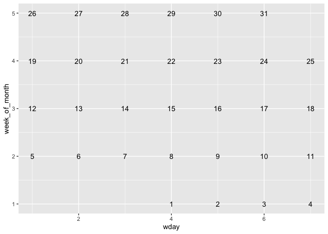
Step 3. Let’s write a user-facing function stat_calendar()
knitrExtra:::chunk_to_r("a_stat_calendar")
stat_calendar <- function(mapping = NULL,
                          data = NULL,
                          geom = "text",
                          position = "identity",
                          na.rm = FALSE,
                          show.legend = NA,
                          inherit.aes = TRUE, ...) {
  ggplot2::layer(
    stat = StatCalendar, # proto object from Step 2
    geom = geom, # inherit other behavior
    data = data,
    mapping = mapping,
    position = position,
    show.legend = show.legend,
    inherit.aes = inherit.aes,
    params = list(na.rm = na.rm, ...)
  )
}
Test stat_calendar
df_year() |>
  ggplot() +
  aes(date = date) +
  stat_calendar(color = "grey") +
  facet_wrap(~month(date, label = T,  abbr = T)) +
  scale_y_reverse()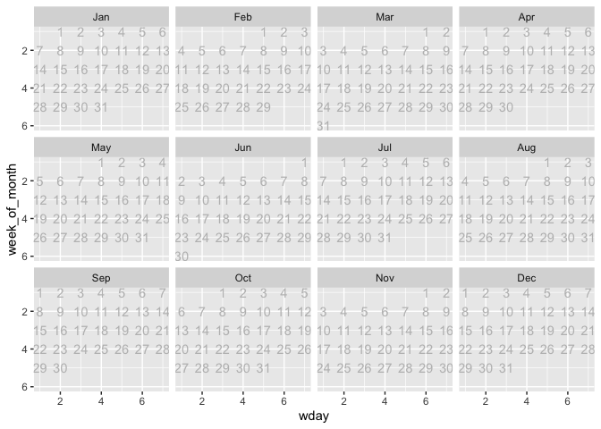
aliasing and convenience
To give the user a better sense of what they’ll see when using stat_calendar we create the alias, ‘geom_text_calendar()’.
knitrExtra:::chunk_to_r("geom_text_calendar")
geom_text_calendar <- stat_calendar
geom_point_calendar <- function(...){stat_calendar(geom = "point", ...)}
geom_tile_calendar <- function(...){stat_calendar(geom = "tile", ...)}
defaults_calendar & ggcalendar() Thinking about set of scales/coords etc, that gives you a nice calendar (to wrap up into defaults)
In our test of stat_calendar, we see cumbersomeness. Below, we consider even more ggplot2 decision that would make our plot easier to consume and more beautiful.
day_labels = c("S", "M", "T", "W", "T", "F", "S")

df_year() |>
  ggplot() +
  aes(date = date) +
  stat_calendar(color = "grey") +
    ggplot2::aes(date = date) +
    ggplot2::scale_y_reverse(breaks = 5:0,
                             expand = c(0,0),
                             limits = c(6.5, 0.5)) +
    ggplot2::scale_x_continuous(breaks = 1:7,
                                labels = day_labels,
                                limits = c(.5, 7.5),
                                expand = c(0,0)
                                ) +
    ggplot2::facet_wrap(~lubridate::month(date, abbr = T, label = T), scales = "free") +
    ggplot2::labs(x = NULL, y = NULL) +
    ggplot2::theme(axis.text.y = ggplot2::element_blank(),
          axis.ticks.y = ggplot2::element_blank(),
          axis.ticks.x = ggplot2::element_blank()) +
    ggplot2::theme(panel.grid.major = ggplot2::element_blank()) +
    ggplot2::geom_blank()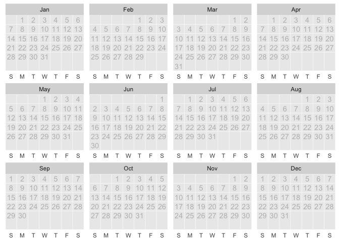
defaults_calendar & ggcalendar()
Then, we bundle these up into defaults_calendar, which can be quickly added for converting to a more polished and readable calendar.
knitrExtra:::chunk_to_r("defaults_calendar")
defaults_calendar <- function(day_labels = c("S", "M", "T", "W", "T", "F", "S")){

  list(
    ggplot2::scale_y_reverse(breaks = 6:0,
                             expand = c(0,0),
                             limits = c(6.5, 0.5)),
    ggplot2::scale_x_continuous(breaks = 1:7,
                                labels = day_labels,
                                limits = c(.5, 7.5),
                                expand = c(0,0)
                                ),
    ggplot2::facet_wrap(~lubridate::month(date, abbr = T, label = T), scales = "free"),
    ggplot2::labs(x = NULL, y = NULL),
    ggplot2::theme(axis.text.y = ggplot2::element_blank(),
          axis.ticks.y = ggplot2::element_blank(),
          axis.ticks.x = ggplot2::element_blank()) +
    ggplot2::theme(panel.grid.major = ggplot2::element_blank()),
    ggplot2::geom_blank()
  )

}
Let’s check it out…
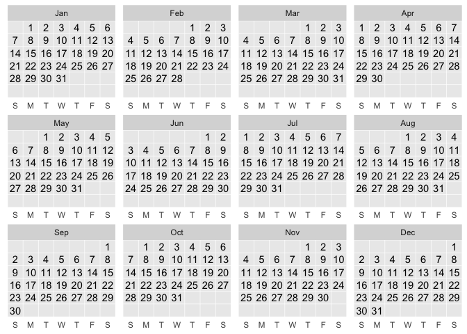
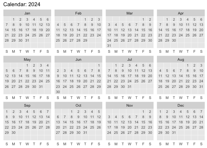
Furthermore, we provide ggcalendar as an alternative point of entry into the ggplot framework. The default data frame is even included (the current calendar year), so a full calendar will print with no additional specification.
knitrExtra:::chunk_to_r("ggcalendar")
ggcalendar <- function(dates_df = df_year(),
                       day_labels = c("S", "M", "T", "W", "T", "F", "S"),
                       labels_layer = TRUE,
                       color = "grey35",
                       size = 3,
                       alpha = .5){

  if(labels_layer){my_layer <- stat_calendar(color = color, aes(date = date), size = size, show.legend = F)}else{my_layer <- NULL}

  ggplot2::ggplot(data = dates_df) +
  defaults_calendar(day_labels = day_labels) +
  ggplot2::aes(date = date) +
  my_layer

  }
Let’s check it out!
ggcalendar()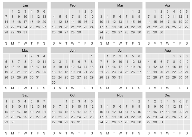
ggcalendar() +
  stat_calendar(geom = "point",
                data = df_week(),
                color = "darkred",
                size = 5,
                alpha = .5)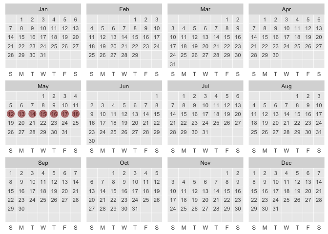
More
library(magrittr)
ggcalendar() +
   # remember default data in ggcalendar() is current year of dates
  aes(date = date) +
  geom_tile_calendar(data = . %>%
                      filter(wday(date) == 3),
                      fill = "blue",
                      alpha = .2) +
  labs(title = "When to do #TidyTuesday in 2024") +
  stat_calendar(label = "X",
                color = "darkred",
                size = 5,
                data = df_dates_interval(
                  "2024/01/01", Sys.Date() - days(1)),
                 alpha = .35)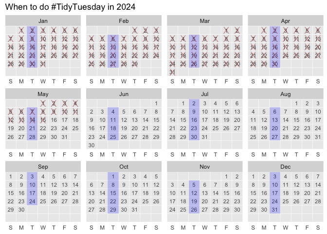
df_month(year = 2023, month = 2) |>
  ggcalendar()
df_month(year = 2023, month = 2) |>
ggcalendar()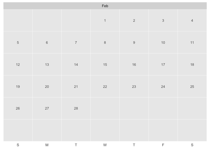
df_month(year = 2023, month = 2) |>
ggcalendar(labels_layer = F) +
  aes(date = date) +
  geom_text_calendar(label = "Another\nday...", # override default
                     size = 4)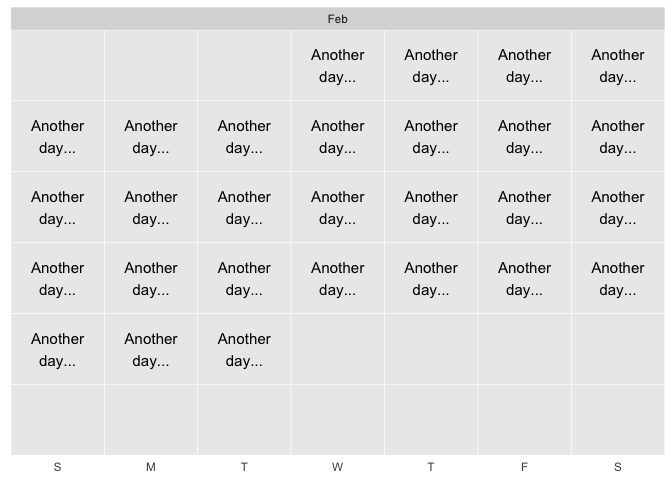
df_month(year = 2023, month = 2) |>
ggcalendar() +
  aes(date = date) +
  geom_text_calendar() +
  geom_point_calendar(data = . %>% filter(wday(date) %in% 2:6),
                      alpha = .2,
                      size = 5,
                      color = "cadetblue") +
  theme(panel.background = element_rect(fill = "beige"))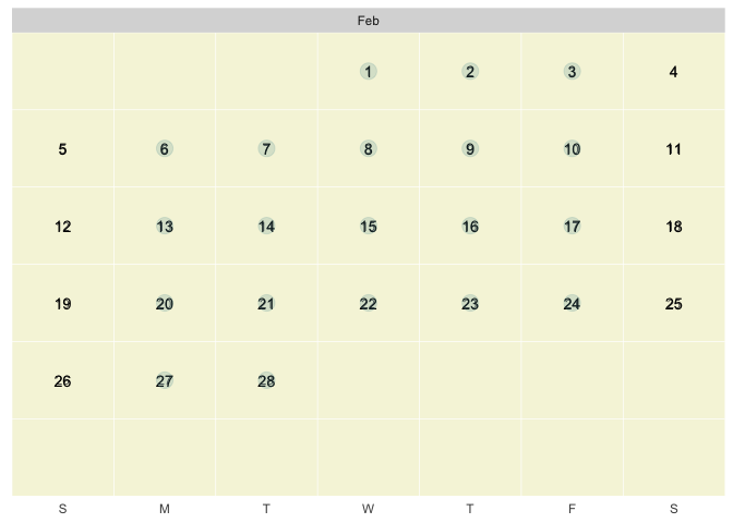
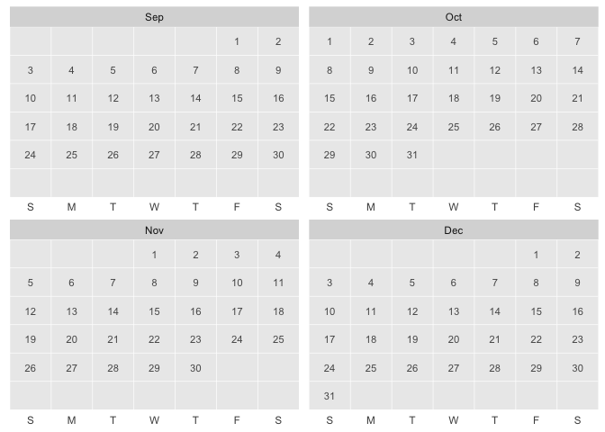
## basic example code
c("2022-03-19", "2022-04-09", "2022-05-07",
  "2022-06-11", "2022-07-16") %>%
  tibble(date = .) |>
  mutate(date = date %>% as_date) |>
  mutate(future = Sys.Date() < date) ->
events

df_year(2022) |>
  ggcalendar() +
  aes(date = date) +
  geom_text_calendar() +
  geom_point_calendar(data = events,
                      aes(color = future),
                      size = 8,
                      alpha = .5,
                      show.legend = F) +
  labs(title = "nu2ggplot2X^2sion, 2022")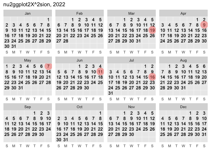
NYC flights Example
Airline on-time data for all flights departing NYC in 2013. Also includes useful ‘metadata’ on airlines, airports, weather, and planes.
Data inspiration: https://twitter.com/rappa753/status/1545729747774308354 @rappa753
# example
nycflights13::flights |>
  ungroup() |>
  mutate(date = as.Date(time_hour)) |>
  filter(year(date) == 2013) |>
  count(date) |>
  ggcalendar() +
  aes(date = date) +
  geom_point_calendar(data = . %>% tibble(), aes(size = n,
                          color = n),
                      alpha = .7, show.legend = F) +
  scale_color_viridis_c(option = "inferno", direction = 1) +
  scale_size(range = c(3,8)) +
  geom_text_calendar(aes(label = n), size = 2) +
  NULL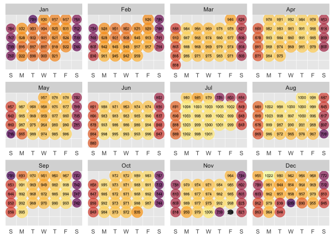
Births example
births <- "https://raw.githubusercontent.com/EvaMaeRey/tableau/9e91c2b5ee803bfef10d35646cf4ce6675b92b55/tidytuesday_data/2018-10-02-us_births_2000-2014.csv"

readr::read_csv(births) |>
  mutate(month = stringr::str_pad(month, 2, pad = "0"),
         date_of_month = str_pad(date_of_month, 2, pad = "0")) |>
  mutate(date = paste(year, month, date_of_month, sep = "-") |> as_date()) |>
  filter(year == 2012) |>
  ggcalendar() +
  aes(date = date) +
  geom_point_calendar(alpha = .4) +
  aes(size = births) +
  aes(color = births) +
  scale_color_viridis_c() +
  guides(
    colour = guide_legend("Births"),
    size = guide_legend("Births")
 ) +
  geom_point_calendar(data = data.frame(date =
                                      as_date("2012-12-25")),
                      size = 5, color = "red", shape = 21)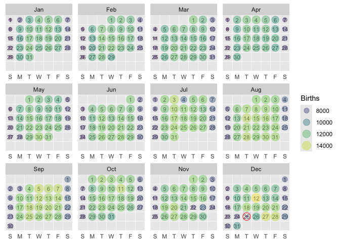
data defaults to calendar year and aes(date = date)
The following feels a little weird to me, but is allowed.
A grammar of graphics fundamental is that a statistical graphic are composed of geometries/marks that take on aesthetics (color, position, size), to represent a variable.
Below we aren’t aren’t fully stating these specifications; which feels a bit funny; I would not recommend this as a starting point.
ggcalendar() +
 geom_text_calendar()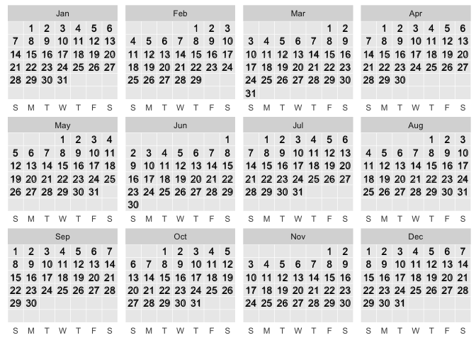
contrast <- function(colour) {
  out   <- rep("grey35", length(colour))
  light <- farver::get_channel(colour, "l", space = "hcl")
  out[light < 50] <- "grey80"
  out
}

aes_autocontrast_color_on_fill <- aes(colour = after_scale(contrast(fill)))


nhl_player_births <- readr::read_csv('https://raw.githubusercontent.com/rfordatascience/tidytuesday/master/data/2024/2024-01-09/nhl_player_births.csv')


nhl_player_births |>
  mutate(date = birth_date %>%
           str_replace("....", "2024") %>%
           as_date()) %>%
  count(date) %>%
  ggcalendar(labels_layer = F) +  # aes(date = date)  # local aes?
  aes(fill = n, label = n) +
  aes_autocontrast_color_on_fill +
  geom_tile_calendar(alpha = .85, linewidth = 0, show.legend = F) +
  scale_fill_viridis_c() +
  geom_text_calendar(size = 3) +
  labs(title = "Number of NHL Player Birthdays by day 1879-2005\nas celebrated in 2024")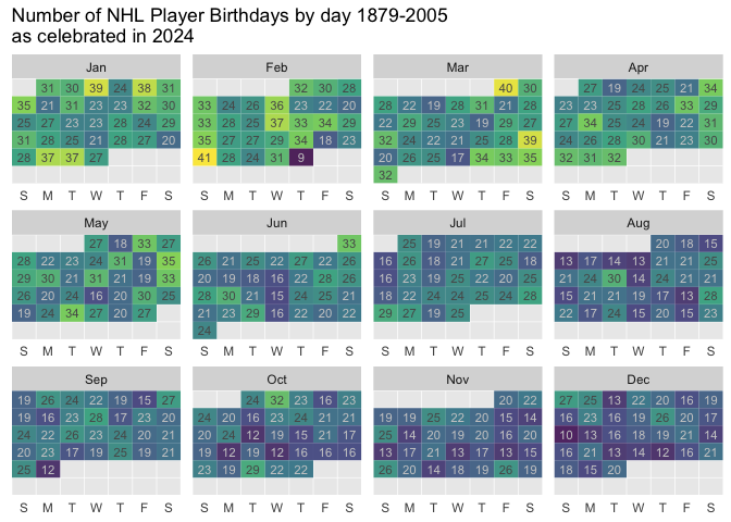
Minimal Viable Packaging
# devtools::create(".")
usethis::use_package("lubridate")
usethis::use_package("ggplot2")
usethis::use_package("dplyr")
usethis::use_package("stringr")

devtools::check()
Traditional README
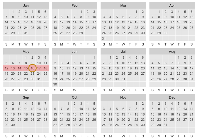
ggcalendar:::ggcalendar() +
  ggcalendar:::geom_tile_calendar(
    data = ggcalendar:::df_week(),
    fill = "red",
    alpha = .25) +
  ggcalendar:::geom_point_calendar(
    data = ggcalendar:::df_today(),
    color = "goldenrod3", shape = 21,
    size = 8, stroke = 1.5
    )
# example
nycflights13::flights |>
  ungroup() |>
  mutate(date = as.Date(time_hour)) |>
  filter(year(date) == 2013) |>
  count(date) |>
  ggcalendar:::ggcalendar(labels_layer = FALSE) +
      aes(date = date) +
      ggcalendar:::geom_tile_calendar(
        aes(fill = n),
        alpha = .7, show.legend = F) +
      scale_fill_viridis_c(option = "inferno",
                            direction = 1) +
      scale_size(range = c(3,8)) +
      ggcalendar:::geom_text_calendar(aes(label = n),
                                      size = 2) +
      NULL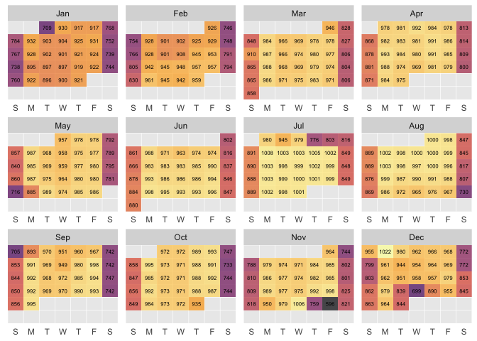
## basic example code
ggcalendar:::df_month(month = "2022-07") |>
  head()

ggcalendar::return_dates_interval(start_date = "2022-07-01", end_date = "2022-08-31") |>
  ggcalendar() +
  aes(date = date) +
  geom_text_calendar(size = 8) +
  geom_point_calendar(data = . %>% filter(date == "2022-07-04"),
                      size = 8,
                      alpha = .5) +
  geom_point_calendar(data = . %>% filter(date < Sys.Date()),
                      size = 10, shape = "x")
more ideas
#' #' Title
#' #'
#' #' @param data
#' #' @param scales
#' #'
#' #' @return
#' #' @export
#' #'
#' #' @examples
#' #' return_dates_year(1999) %>%
#' #' head() %>%
#' #' compute_group_calendar()
#' #'
#' compute_group_weekly <- function(data, scales){
#'
#'   data %>%
#'     dplyr::mutate(num_day_of_week = lubridate::wday(.data$date)) %>%
#'     dplyr::mutate(day_of_week = lubridate::wday(.data$date, label = TRUE, abbr = TRUE)) %>%
#'     dplyr::mutate(week_of_month = (- lubridate::wday(.data$date) + lubridate::day(.data$date)) %/% 7 + 1 +
#'                     ifelse(lubridate::wday(lubridate::floor_date(lubridate::as_date(.data$date), "month")) == 1, -1, 0)
#'                   ) %>%
#'     dplyr::mutate(date_of_month = lubridate::day(.data$date)) %>%
#'     dplyr::mutate(which_year = lubridate::year(.data$date) - 2018) %>%
#'     dplyr::mutate(month = lubridate::month(.data$date, abbr = TRUE, label = TRUE)) %>%
#'     dplyr::mutate(hour = lubridate::hour(.data$date)) %>%
#'     dplyr::mutate(academic_year =  lubridate::year(.data$date) +
#'                     ifelse(lubridate::month(date) >
#'                              6, 1, 0)) %>%
#'     dplyr::mutate(academic_month = .data$month %>%
#'                     factor(levels = c("Jul", "Aug", "Sep", "Oct", "Nov", "Dec",
#'                                       "Jan", "Feb", "Mar", "Apr", "May", "Jun")))
#'
#' }
#'
#' StatWeekly <- ggplot2::ggproto(`_class` = "StatWeekly",
#'                                  `_inherit` = ggplot2::Stat,
#'                                  required_aes = c("date"),
#'                                  compute_group = compute_group_weekly,
#'                                  default_aes = ggplot2::aes(x = ggplot2::after_stat(day_of_week %>% as.numeric()),
#'                                                             y = ggplot2::after_stat(hour),
#'                                                             label = ggplot2::after_stat(date_of_month)))
#'
#' Title
#'
#' @param dates_df
#'
#' @return
#' @export
#'
#' @examples
#' library(lubridate)
#' library(dplyr)
#' library(ggplot2)
#' library(magrittr)
#'
#' ggweekly() +
#' geom_text_weekly()
#'
#' ggweekly() +
#' geom_text_weekly(color = "grey35") +
#' labs(title = "When to do #TidyTuesday in 2022") +
#' geom_text_weekly(label = "X",
#'                   data = data.frame(date = seq(as.Date("2022/01/01"),
#'                   as.Date("2022/04/18"), "days")))
#'
ggweekly <- function(dates_df = return_hours_week(), day_labels = c("S", "M", "T", "W", "T", "F", "S")){


  ggplot2::ggplot(data = dates_df) +
    ggplot2::aes(date = date) +
    ggplot2::scale_y_reverse(
      breaks = 7:21,
                             expand = c(0,0),
                             limits = c(21 + .5,
                                        7 - .5),

                             ) +
    ggplot2::scale_x_continuous(breaks = 1:7, labels = day_labels,
                                limits = c(.5, 7.5),expand = c(0,0)

                                #position = "top"
                                ) +
    ggplot2::facet_wrap(~epiweek(date), scales = "free") +
    ggplot2::labs(x = NULL, y = NULL) +
    ggplot2::theme(#axis.text.y = ggplot2::element_blank(),
          axis.ticks.y = ggplot2::element_blank(),
          axis.ticks.x = ggplot2::element_blank()) +
    ggplot2::theme(panel.grid.major = ggplot2::element_blank()) +
    ggplot2::geom_blank() +
    # theme(strip.placement = "outside") +
    NULL

}