ggdims
- ggdims Intro Thoughts
- Supporting work and discussions
- examples…
- Applications: tsne, umap, PCA
- Minimal Packaging
- Reproduction exercise
Go to talk
ggdims Intro Thoughts
ggplot2 lets you intuitively translate variables to visual
representation. You specify how variables (e.g. sex, age, employment
status) are to be communicated via visual channels (x and y axis
position, color, transparency, etc). However, in ggplot2 these
specifications are individual-variable-to-individual-visual-channel
which does not lend itself easily to visualizations in the world of
dimension reduction (e.g. PCA, t-SNE, umap). The usual
one-var-to-one-aesthetic requirement means that it may not feel obvious
how to extend ggplot2 for dimensionality reduction visualization, which
deals with characterizing many variables. So while using ggplot2
under-the-hood is common in the dim-red space, it feels like there may
be less consistency across dim-red APIs. For users of these APIs,
getting quickly acquainted with techniques (students) or doing
comparative work (practitioners) may be more challenging than it needs
to be. The {ggdims} package explores a new dims() and dims_expand()
utility that could help with greater consistency across dim-red APIs,
with standard ggplots, and within the ggplot2 extension ecosystem.
ggdims proposes the following API:
library(ggplot2)

ggplot(data = my_high_dimensional_data) +
  aes(dims = dims(var1:var200, var205)) +      # or similar
  geom_reduction_technique()                 # default dim-red to 2D

last_plot() +
  aes(color = label)    # indicate category
Supporting work and discussions
Here, doing some further thinking about a dimensionality reduction framework for ggplot2. Based on some previous work: 2025-07-18, 2025-08-19, 2025-10-11 and discussions ggplot-extension-club/discussions/117 and ggplot-extension-club/discussions/18
library(tidyverse)
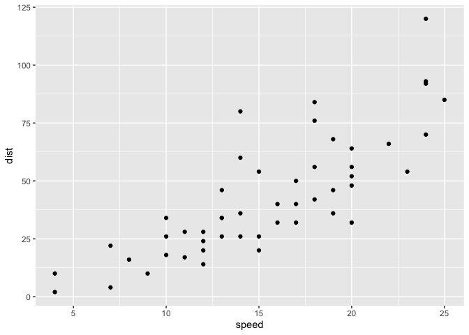
ggplot(data = cars) +
aes(x = speed, y = dist) ->
data_and_vars_plot_specs
data_and_vars_plot_specs +
geom_point()
examples…
#> [1] "rc9143" "rc9144" "rc9145" "rc9146" "rc9147" "continent"
library(ggdims)
unga_rcid_wide[1:5, 1:5]
#> # A tibble: 5 × 5
#> country country_code rc3 rc4 rc5
#> <chr> <chr> <dbl> <dbl> <dbl>
#> 1 United States US 1 0 0
#> 2 Canada CA 0 0 0
#> 3 Cuba CU 1 0 1
#> 4 Haiti HT 1 0 0
#> 5 Dominican Republic DO 1 0 0
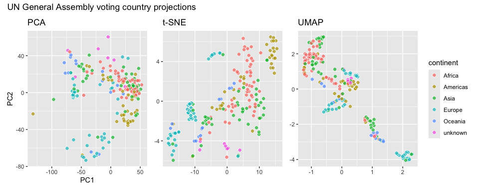
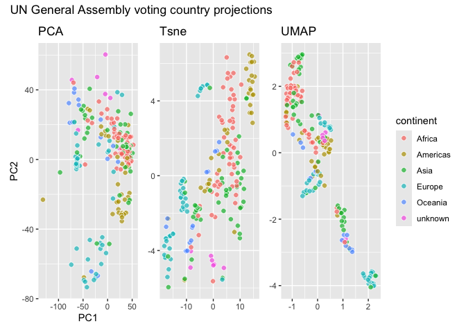
unga_pca <- unga_rcid_wide |>
ggplot() +
aes(dims = dims(rc3:rc9147)) +
geom_pca() +
aes(fill = continent) +
labs(title = "PCA")
unga_tsne <- ggplot(unga_rcid_wide) +
  aes(dims = dims(rc3:rc9147)) +
  geom_tsne() +
  aes(fill = continent) +
  labs(title = "t-SNE")
unga_umap <-
  ggplot(unga_rcid_wide) +
  aes(dims = dims(rc3:rc9147)) +
  geom_umap() +
  aes(fill = continent) +
  labs(title = "UMAP")
library(patchwork)
unga_pca + unga_tsne + unga_umap +
  plot_layout(guides = "collect") +
  plot_annotation(title = "UN General Assembly voting country projections")
This is in the experimental/proof of concept phase. 🤔🚧
An implementation
so let’s use some ggplot_add to try to expand, and have these individually specified vars
 ``` r
p <- last_plot()
p$mapping$dims[[2]] # the unexpanded expression
#> dims(Sepal.Length:Petal.Length, Petal.Width)
p$mapping$dims |>
as.character() |>
_[2] |>
stringr::str_extract("\\(.+") |>
stringr::str_remove_all("\\(|\\)") ->
selected_var_names_expr
selected_var_names <-
selected_var_names_expr |>
str_split(", ") |>
_[[1]]
var_names <- c()
for(i in 1:length(selected_var_names)){
new_var_names <- select(last_plot()$data, !!!list(rlang::parse_expr(selected_var_names[i]))) |> names()
var_names <- c(var_names, new_var_names)
}
expanded_vars <- var_names |> paste(collapse = ", ")
new_dim_expr <- paste("dims_listed(", expanded_vars, ")")
p$mapping <- modifyList(p$mapping, aes(dims0 = pi()))
p$mapping$dims0[[2]] <- rlang::parse_expr(new_dim_expr)
p$mapping$dims0[[2]]
#> dims_listed(Sepal.Length, Sepal.Width, Petal.Length, Petal.Width)
```
``` r
p <- last_plot()
p$mapping$dims[[2]] # the unexpanded expression
#> dims(Sepal.Length:Petal.Length, Petal.Width)
p$mapping$dims |>
as.character() |>
_[2] |>
stringr::str_extract("\\(.+") |>
stringr::str_remove_all("\\(|\\)") ->
selected_var_names_expr
selected_var_names <-
selected_var_names_expr |>
str_split(", ") |>
_[[1]]
var_names <- c()
for(i in 1:length(selected_var_names)){
new_var_names <- select(last_plot()$data, !!!list(rlang::parse_expr(selected_var_names[i]))) |> names()
var_names <- c(var_names, new_var_names)
}
expanded_vars <- var_names |> paste(collapse = ", ")
new_dim_expr <- paste("dims_listed(", expanded_vars, ")")
p$mapping <- modifyList(p$mapping, aes(dims0 = pi()))
p$mapping$dims0[[2]] <- rlang::parse_expr(new_dim_expr)
p$mapping$dims0[[2]]
#> dims_listed(Sepal.Length, Sepal.Width, Petal.Length, Petal.Width)
```
dims_expand
See also a new approach ??
p <- iris |>
  ggplot() +
  aes(dims = dims(Sepal.Length:Petal.Length, Petal.Width)) +
  dims_expand()


p$mapping
#> Aesthetic mapping:
#> * `dims` -> `dims_listed(Sepal.Length, Sepal.Width, Petal.Length, Petal.Width)`
Now let’s actually define dims_listed() and vars_unpack
Applications: tsne, umap, PCA
compute_tsne, geom_tsne, using Rtsne::Rtsne
 ``` r
p$mapping$dims
#>
``` r
p$mapping$dims
#>  ``` r
#' @export
theme_ggdims <- function(ink = "black", paper = "white"){
theme_grey() +
theme(panel.background = element_blank(),
panel.grid = element_blank(),
axis.text = element_blank(),
axis.ticks = element_blank(),
panel.border = element_rect(color = ink)
)
}
```
``` r
#' @export
geom_tsne <- function(...){
list(
dims_expand(),
geom_tsne0(...)
)
}
#' @export
geom_tsne_label <- function(...){
list(
dims_expand(),
geom_tsne_label0(...)
)
}
```
</details>
``` r
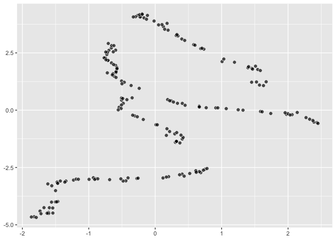
iris |>
ggplot() +
aes(dims = dims(Sepal.Length:Petal.Length, Petal.Width)) +
geom_tsne()
```
``` r
#' @export
theme_ggdims <- function(ink = "black", paper = "white"){
theme_grey() +
theme(panel.background = element_blank(),
panel.grid = element_blank(),
axis.text = element_blank(),
axis.ticks = element_blank(),
panel.border = element_rect(color = ink)
)
}
```
``` r
#' @export
geom_tsne <- function(...){
list(
dims_expand(),
geom_tsne0(...)
)
}
#' @export
geom_tsne_label <- function(...){
list(
dims_expand(),
geom_tsne_label0(...)
)
}
```
</details>
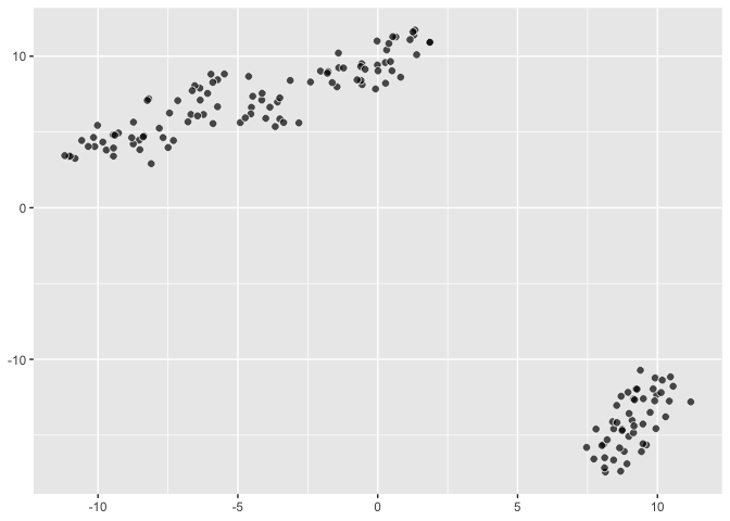
``` r
iris |>
ggplot() +
aes(dims = dims(Sepal.Length:Petal.Length, Petal.Width)) +
geom_tsne()
```
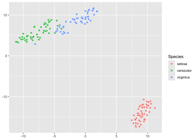
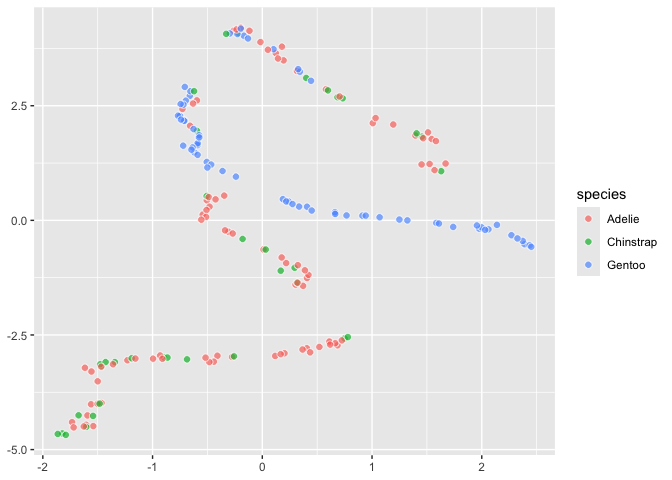
 ``` r
last_plot() +
aes(fill = Species)
```
``` r
last_plot() +
aes(fill = Species)
```
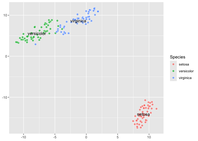
 ``` r
last_plot() +
aes(label = Species) +
geom_tsne_label()
```
``` r
last_plot() +
aes(label = Species) +
geom_tsne_label()
```
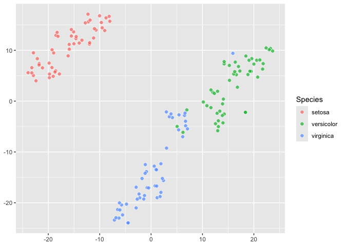
 ### Different perplexity
``` r
iris |>
ggplot() +
aes(dims = dims(Sepal.Length:Petal.Length, Petal.Width),
fill = Species) +
geom_tsne(perplexity = 10)
```
### Different perplexity
``` r
iris |>
ggplot() +
aes(dims = dims(Sepal.Length:Petal.Length, Petal.Width),
fill = Species) +
geom_tsne(perplexity = 10)
```
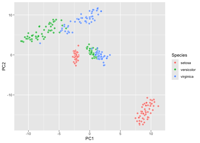
 ## A little UMAP using [`umap::umap`](https://github.com/tkonopka/umap)
 ``` r
last_plot() +
aes(fill = Species)
```
``` r
last_plot() +
aes(fill = Species)
```
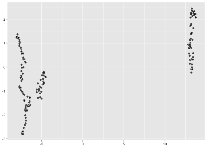
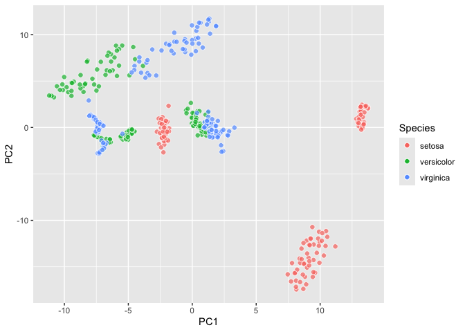
 ## A little PCA using `ordr::ordinate`
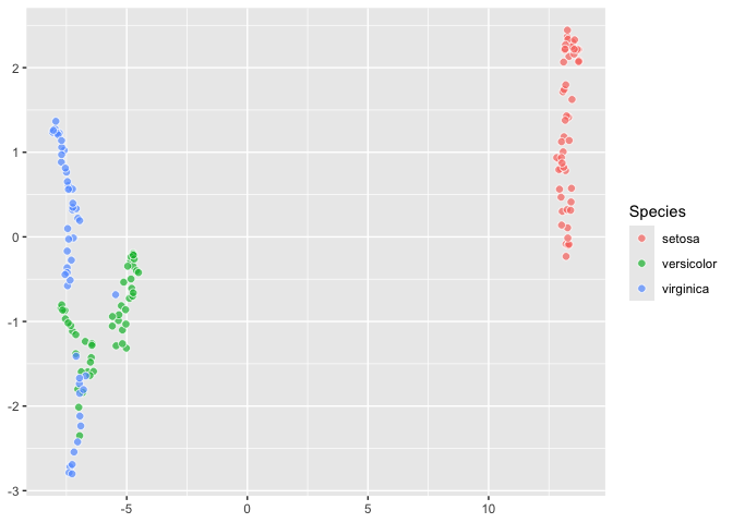
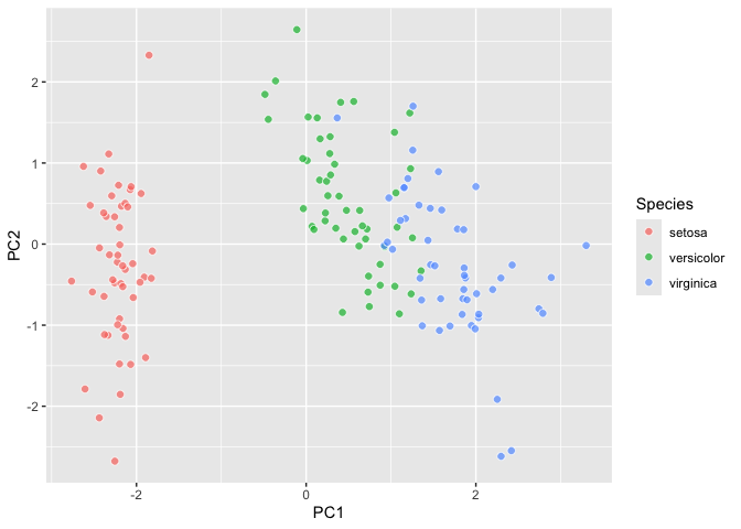
 ``` r
last_plot() +
aes(fill = Species)
```
``` r
last_plot() +
aes(fill = Species)
```
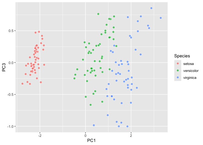
 ``` r
last_plot() +
aes(y = after_stat(PC3))
```
``` r
last_plot() +
aes(y = after_stat(PC3))
```
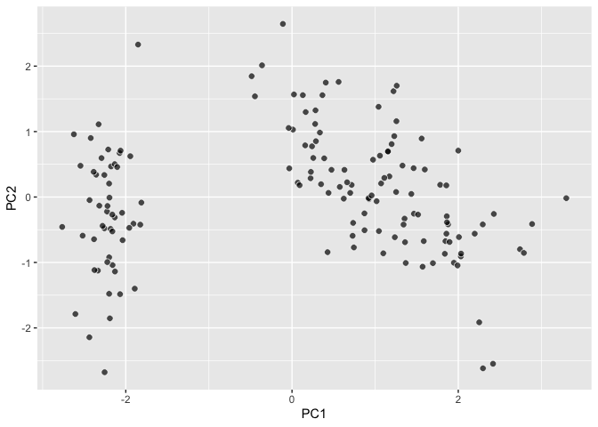
 ``` r
library(ggdims)
iris |>
ggplot() +
aes(dims = dims(Sepal.Length:Petal.Width)) +
geom_pca() +
aes(fill = Species) ->
iris_pca; iris_pca
```
``` r
library(ggdims)
iris |>
ggplot() +
aes(dims = dims(Sepal.Length:Petal.Width)) +
geom_pca() +
aes(fill = Species) ->
iris_pca; iris_pca
```
 ``` r
ggplyr::last_plot_wipe() +
geom_tsne() ->
iris_tsne; iris_tsne
```
``` r
ggplyr::last_plot_wipe() +
geom_tsne() ->
iris_tsne; iris_tsne
```
 ``` r
ggplyr::last_plot_wipe() +
geom_umap() ->
iris_umap; iris_umap
```
``` r
ggplyr::last_plot_wipe() +
geom_umap() ->
iris_umap; iris_umap
```
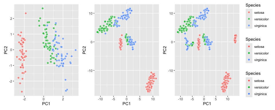
 ``` r
library(patchwork)
iris_pca + iris_tsne + iris_umap + patchwork::plot_layout(guides = "collect")
```
``` r
library(patchwork)
iris_pca + iris_tsne + iris_umap + patchwork::plot_layout(guides = "collect")
```
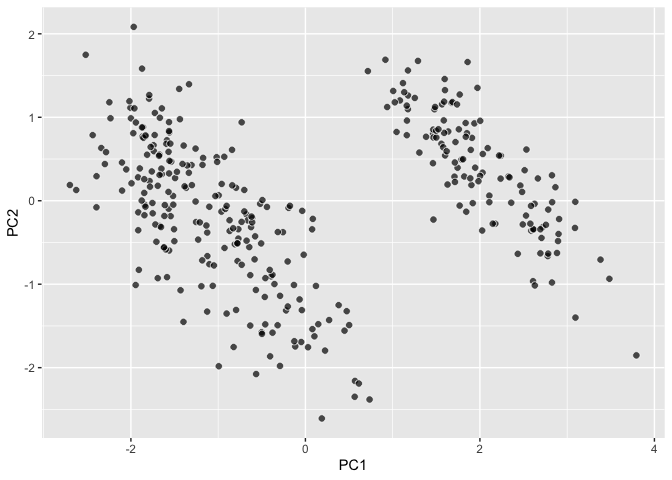
 ### w/ penguins
``` r
palmerpenguins::penguins |>
ggplot() +
aes(dims = dims(bill_length_mm:body_mass_g)) +
geom_pca()
```
### w/ penguins
``` r
palmerpenguins::penguins |>
ggplot() +
aes(dims = dims(bill_length_mm:body_mass_g)) +
geom_pca()
```
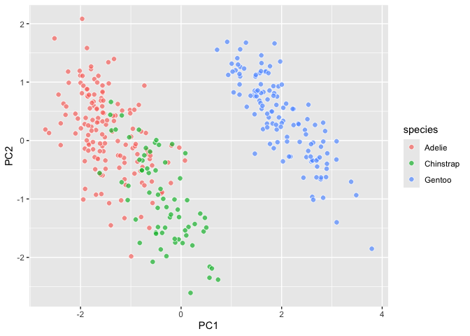
 ``` r
last_plot() +
aes(fill = species)
```
``` r
last_plot() +
aes(fill = species)
```
 # Minimal Packaging
``` r
# knitrExtra::chunk_names_get()
knitrExtra::chunk_to_dir(
c( "dims_expand" , "dims_listed", "data_vars_unpack", "compute_tsne", "theme_ggdims", "geom_tsne", "compute_umap", "compute_pca_rows", "aaa_GeomPointFill" )
)
usethis::use_package("ggplot2")
devtools::document()
```
``` r
devtools::check(".")
devtools::install(".", upgrade = "never")
```
# Reproduction exercise
Try to reproduce some of observations and figures in the Distill paper:
‘How to Use t-SNE Effectively’ <https://distill.pub/2016/misread-tsne/>
with some verbatim visuals from the paper.
``` r
knitr::opts_chunk$set(out.width = NULL, fig.show = "asis")
```
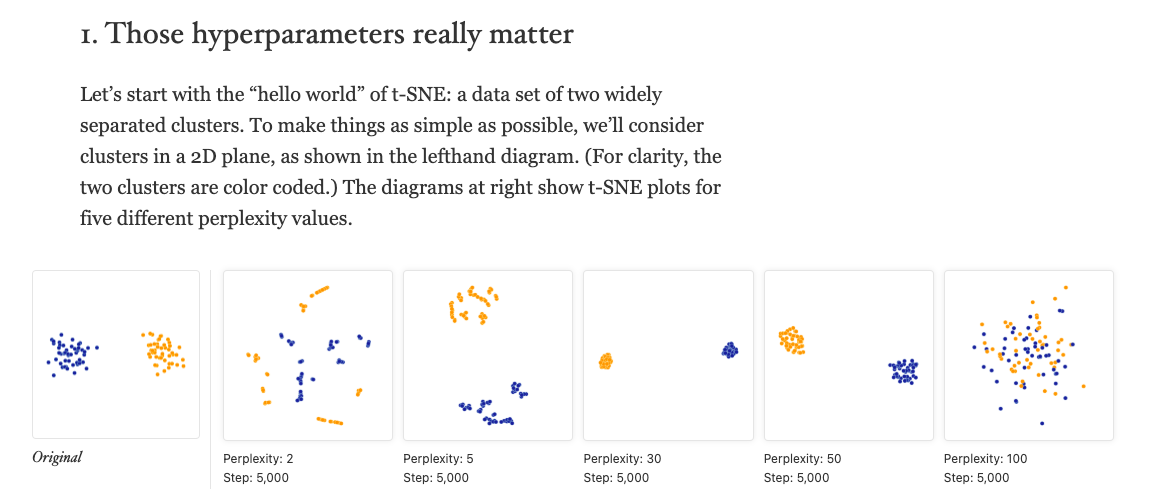
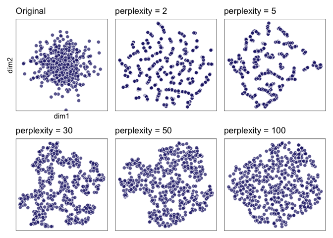
### 1. ‘Those hyperparameters really matter’
# Minimal Packaging
``` r
# knitrExtra::chunk_names_get()
knitrExtra::chunk_to_dir(
c( "dims_expand" , "dims_listed", "data_vars_unpack", "compute_tsne", "theme_ggdims", "geom_tsne", "compute_umap", "compute_pca_rows", "aaa_GeomPointFill" )
)
usethis::use_package("ggplot2")
devtools::document()
```
``` r
devtools::check(".")
devtools::install(".", upgrade = "never")
```
# Reproduction exercise
Try to reproduce some of observations and figures in the Distill paper:
‘How to Use t-SNE Effectively’ <https://distill.pub/2016/misread-tsne/>
with some verbatim visuals from the paper.
``` r
knitr::opts_chunk$set(out.width = NULL, fig.show = "asis")
```
### 1. ‘Those hyperparameters really matter’
 ``` r
two_clusters <- data.frame(dim1 =
rnorm(101, mean = -.5,
sd = .1) |>
c(rnorm(101, mean = .5,
sd = .1)),
dim2 = rnorm(202, sd = .1),
type = c(rep("A", 101), rep("B", 101)))
big_and_small_cluster <- data.frame(dim1 = c(rnorm(100, -.5, sd = .1),
rnorm(100, .7, sd = .03)),
dim2 = c(rnorm(100, sd = .1),
rnorm(100, sd = .03)),
type = c(rep("A", 100), rep("B", 100)))
two_close_and_one_far <- data.frame(dim1 =
c(rnorm(150, -.75, .05),
rnorm(150, -.35, .05),
rnorm(150, .75, .05)),
dim2 = rnorm(450, sd = .05),
type = c(rep("A", 150),
rep("B", 150),
rep("C", 150)))
random_noise <- data.frame(dim1 = rnorm(500, sd = .3),
dim2 = rnorm(500, sd = .3),
type = "A")
```
``` r
usethis::use_data(two_clusters, overwrite = T)
usethis::use_data(big_and_small_cluster, overwrite = T)
usethis::use_data(two_close_and_one_far, overwrite = T)
usethis::use_data(random_noise, overwrite = T)
```
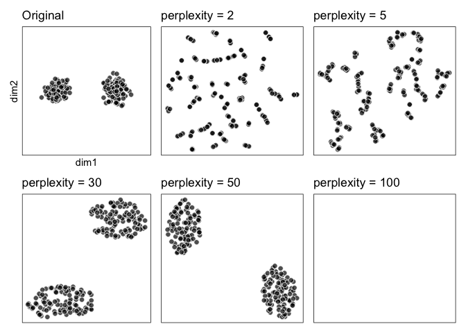
Let’s try to reproduce the following with our `geom_tsne()`:
``` r
dim(two_clusters)
#> [1] 202 3
original <- two_clusters |>
ggplot() +
aes(x = dim1,
y = dim2) +
geom_point(shape = 21, color = "white",
alpha = .7,
aes(size = from_theme(pointsize * 1.5))) +
labs(title = "Original") +
aes(fill = I("black")) +
coord_equal(xlim = c(-1,1), ylim = c(-1,1))
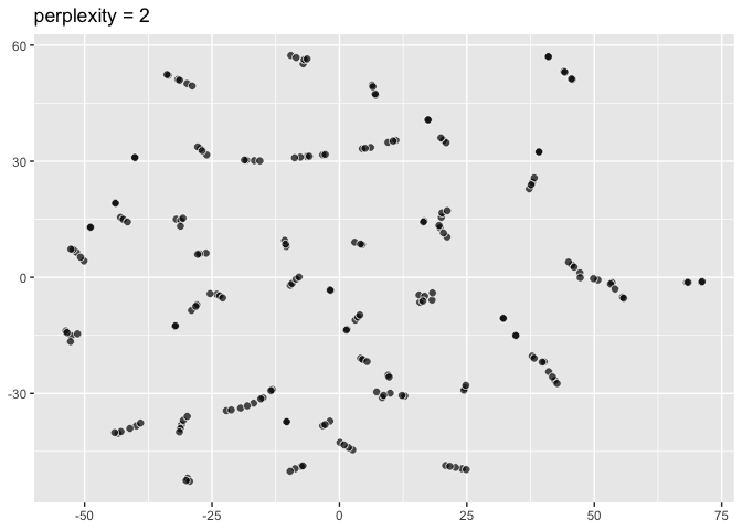
pp2 <- ggplot(data = two_clusters) +
aes(dims = dims(dim1:dim2)) +
geom_tsne(perplexity = 2) +
labs(title = "perplexity = 2"); pp2
```
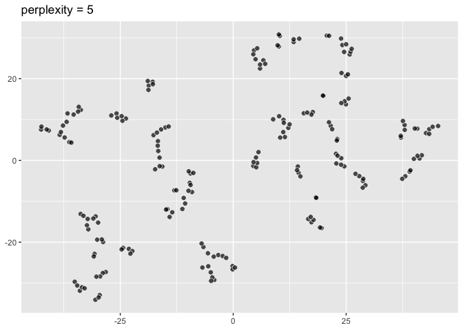
``` r
pp5 <- ggplot(data = two_clusters) +
aes(dims = dims(dim1:dim2)) +
geom_tsne(perplexity = 5) +
labs(title = "perplexity = 5"); pp5
```
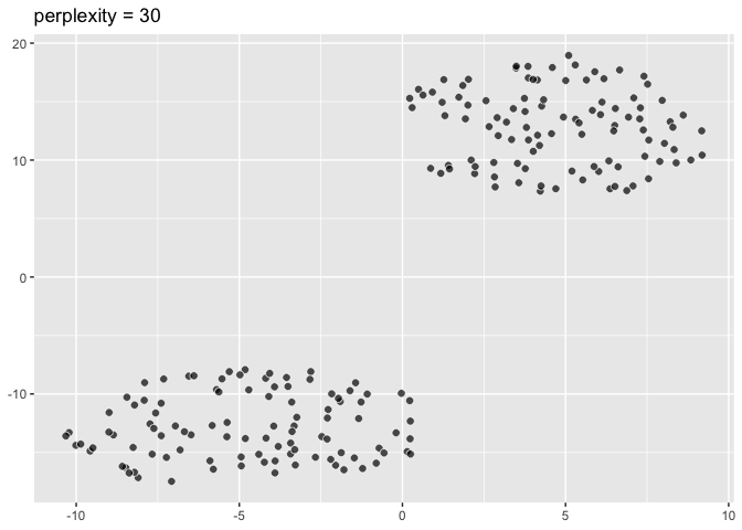
``` r
pp30 <- ggplot(data = two_clusters) +
aes(dims = dims(dim1:dim2)) +
geom_tsne(perplexity = 30) +
labs(title = "perplexity = 30"); pp30
```
``` r
pp50 <- ggplot(data = two_clusters) +
aes(dims = dims(dim1:dim2)) +
geom_tsne(perplexity = 50) +
labs(title = "perplexity = 50")
pp100 <- ggplot(data = two_clusters) +
aes(dims = dims(dim1:dim2)) +
geom_tsne(perplexity = 100) +
labs(title = "perplexity = 100")
library(patchwork)
original + pp2 + pp5 + pp30 + pp50 + pp100 &
theme_ggdims()
```
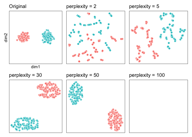
``` r
# with group id
last_plot() &
aes(fill = type) &
guides(fill = "none")
```
``` r
panel_of_six_tsne_two_cluster <- last_plot()
```
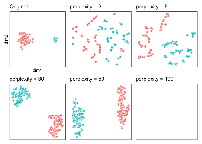
### 2. ‘Cluster sizes in a t-SNE plot mean nothing’
Let’s try to reproduce this (we’ll shortcut but switching out the data
across plot specifications): 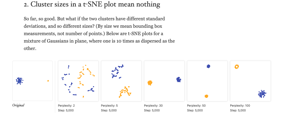
``` r
panel_of_six_tsne_two_cluster &
ggplyr::data_replace(big_and_small_cluster)
```
#### Side note on ggplyr::data_replace X google gemini quick search
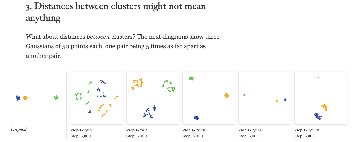
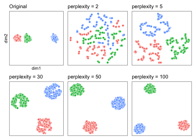
### 3. ‘Distances between clusters might not mean anything’
Now let’s look at these three clusters, where one cluster is far out:
``` r
two_clusters <- data.frame(dim1 =
rnorm(101, mean = -.5,
sd = .1) |>
c(rnorm(101, mean = .5,
sd = .1)),
dim2 = rnorm(202, sd = .1),
type = c(rep("A", 101), rep("B", 101)))
big_and_small_cluster <- data.frame(dim1 = c(rnorm(100, -.5, sd = .1),
rnorm(100, .7, sd = .03)),
dim2 = c(rnorm(100, sd = .1),
rnorm(100, sd = .03)),
type = c(rep("A", 100), rep("B", 100)))
two_close_and_one_far <- data.frame(dim1 =
c(rnorm(150, -.75, .05),
rnorm(150, -.35, .05),
rnorm(150, .75, .05)),
dim2 = rnorm(450, sd = .05),
type = c(rep("A", 150),
rep("B", 150),
rep("C", 150)))
random_noise <- data.frame(dim1 = rnorm(500, sd = .3),
dim2 = rnorm(500, sd = .3),
type = "A")
```
``` r
usethis::use_data(two_clusters, overwrite = T)
usethis::use_data(big_and_small_cluster, overwrite = T)
usethis::use_data(two_close_and_one_far, overwrite = T)
usethis::use_data(random_noise, overwrite = T)
```
Let’s try to reproduce the following with our `geom_tsne()`:
``` r
dim(two_clusters)
#> [1] 202 3
original <- two_clusters |>
ggplot() +
aes(x = dim1,
y = dim2) +
geom_point(shape = 21, color = "white",
alpha = .7,
aes(size = from_theme(pointsize * 1.5))) +
labs(title = "Original") +
aes(fill = I("black")) +
coord_equal(xlim = c(-1,1), ylim = c(-1,1))
pp2 <- ggplot(data = two_clusters) +
aes(dims = dims(dim1:dim2)) +
geom_tsne(perplexity = 2) +
labs(title = "perplexity = 2"); pp2
```

``` r
pp5 <- ggplot(data = two_clusters) +
aes(dims = dims(dim1:dim2)) +
geom_tsne(perplexity = 5) +
labs(title = "perplexity = 5"); pp5
```

``` r
pp30 <- ggplot(data = two_clusters) +
aes(dims = dims(dim1:dim2)) +
geom_tsne(perplexity = 30) +
labs(title = "perplexity = 30"); pp30
```

``` r
pp50 <- ggplot(data = two_clusters) +
aes(dims = dims(dim1:dim2)) +
geom_tsne(perplexity = 50) +
labs(title = "perplexity = 50")
pp100 <- ggplot(data = two_clusters) +
aes(dims = dims(dim1:dim2)) +
geom_tsne(perplexity = 100) +
labs(title = "perplexity = 100")
library(patchwork)
original + pp2 + pp5 + pp30 + pp50 + pp100 &
theme_ggdims()
```

``` r
# with group id
last_plot() &
aes(fill = type) &
guides(fill = "none")
```

``` r
panel_of_six_tsne_two_cluster <- last_plot()
```
### 2. ‘Cluster sizes in a t-SNE plot mean nothing’
Let’s try to reproduce this (we’ll shortcut but switching out the data
across plot specifications): 
``` r
panel_of_six_tsne_two_cluster &
ggplyr::data_replace(big_and_small_cluster)
```

#### Side note on ggplyr::data_replace X google gemini quick search

### 3. ‘Distances between clusters might not mean anything’
Now let’s look at these three clusters, where one cluster is far out:
 ``` r
panel_of_six_tsne_two_cluster &
ggplyr::data_replace(two_close_and_one_far)
```
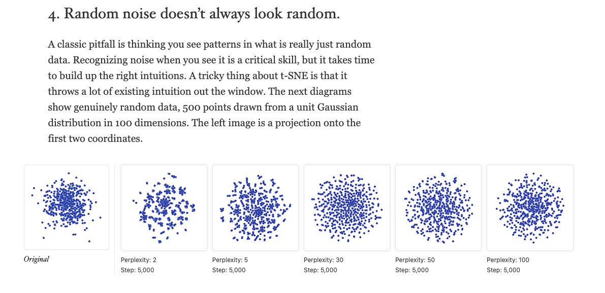
### 4. ‘Random noise doesn’t always look random’
``` r
panel_of_six_tsne_two_cluster &
ggplyr::data_replace(random_noise) &
aes(fill = I("midnightblue"))
```
------------------------------------------------------------------------
``` r
palmerpenguins::penguins |>
sample_n(size = 200) |>
remove_missing() |>
ggplot() +
aes(dims = dims(bill_length_mm:body_mass_g)) +
geom_umap()
```
``` r
last_plot() +
aes(fill = species)
```
``` r
unvotes::un_votes |>
arrange(rcid) |>
mutate(rcid = paste0("rc",rcid) |> fct_inorder()) |>
mutate(num_vote = case_when(vote == "yes" ~ 1,
vote == "abstain" ~ .5,
vote == "no" ~ 0,
TRUE ~ .5 )) |>
# filter(rcid %in% 1:30) |>
pivot_wider(id_cols = c(country, country_code),
names_from = rcid,
values_from = num_vote,
values_fill = .5
) |>
mutate(continent = country_code |>
countrycode::countrycode(origin = "iso2c", destination = "continent")) |>
mutate(continent = continent |> is.na() |> ifelse("unknown", continent)) ->
unga_rcid_wide
names(unga_rcid_wide) |> tail()
#> [1] "rc9143" "rc9144" "rc9145" "rc9146" "rc9147" "continent"
```
``` r
# maybe too big?
# usethis::use_data(unga_rcid_wide, overwrite = T)
```
``` r
dims_specs <-
unga_rcid_wide |>
ggplot() +
aes(dims = dims(rc3:rc9147),
fill = continent)
```
``` r
library(patchwork)
(dims_specs + geom_pca() + labs(title = "PCA")) +
(dims_specs + geom_tsne() + labs(title = "Tsne")) +
(dims_specs + geom_umap() + labs(title = "UMAP")) +
patchwork::plot_layout(guides = "collect") +
plot_annotation(title = "UN General Assembly voting country projections")
```
``` r
panel_of_six_tsne_two_cluster &
ggplyr::data_replace(two_close_and_one_far)
```

### 4. ‘Random noise doesn’t always look random’

``` r
panel_of_six_tsne_two_cluster &
ggplyr::data_replace(random_noise) &
aes(fill = I("midnightblue"))
```

------------------------------------------------------------------------
``` r
palmerpenguins::penguins |>
sample_n(size = 200) |>
remove_missing() |>
ggplot() +
aes(dims = dims(bill_length_mm:body_mass_g)) +
geom_umap()
```

``` r
last_plot() +
aes(fill = species)
```

``` r
unvotes::un_votes |>
arrange(rcid) |>
mutate(rcid = paste0("rc",rcid) |> fct_inorder()) |>
mutate(num_vote = case_when(vote == "yes" ~ 1,
vote == "abstain" ~ .5,
vote == "no" ~ 0,
TRUE ~ .5 )) |>
# filter(rcid %in% 1:30) |>
pivot_wider(id_cols = c(country, country_code),
names_from = rcid,
values_from = num_vote,
values_fill = .5
) |>
mutate(continent = country_code |>
countrycode::countrycode(origin = "iso2c", destination = "continent")) |>
mutate(continent = continent |> is.na() |> ifelse("unknown", continent)) ->
unga_rcid_wide
names(unga_rcid_wide) |> tail()
#> [1] "rc9143" "rc9144" "rc9145" "rc9146" "rc9147" "continent"
```
``` r
# maybe too big?
# usethis::use_data(unga_rcid_wide, overwrite = T)
```
``` r
dims_specs <-
unga_rcid_wide |>
ggplot() +
aes(dims = dims(rc3:rc9147),
fill = continent)
```
``` r
library(patchwork)
(dims_specs + geom_pca() + labs(title = "PCA")) +
(dims_specs + geom_tsne() + labs(title = "Tsne")) +
(dims_specs + geom_umap() + labs(title = "UMAP")) +
patchwork::plot_layout(guides = "collect") +
plot_annotation(title = "UN General Assembly voting country projections")
```
