ggplot2 allows you build up your plot bit by bit – to write ‘graphical poems’ (Wickham 2010). It is easy to gain insights simply by 1. defining a data set to look at, 2. the aesthetics (x position, y position, color, size, etc) that should represent variables from that data, and 3. what geometric marks should take on those aesthetics. Inspired by this incrementalism, frameworks like camcorder, flipbookr, codehover exist to capture plot composition.
Here is a graphical poem!
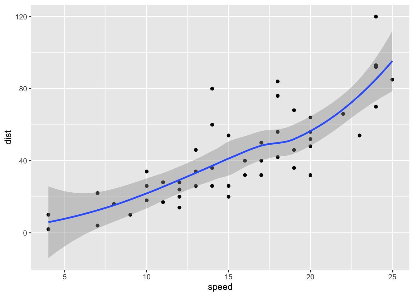
ggplot(data = cars) +# The first declaration you typically make is the dataframe to plotaes(x = speed, y = dist) +# The second declaration is what visual channels should represent which variables (here x and y position are used to represent speed and distance)geom_point() +# Then you'll specify the mark (point here) that will take on the aesthetics (x or y position here, but color, size, shape are other examples)geom_smooth() # Finally we might be interested in making some predictions; what is the expected value (mean) of y given some x (here stopping distance given some speed upon breaking)
Closeread helps walk people through and digest ideas suggesting a synergy with the gg world. With Closereads, maybe we can read this graphical poem ‘aloud’, and reflect on it a bit in plain language as we go. Here is a generic way to write out what closereads requires for creating plot output and referring to it.
cr_last_plot_construction <-':::{focus-on="cr-.PLOTXXX"}\n.COMMENT, using `.CODE`\n:::\n\n:::{#cr-.PLOTXXX}\n```{r .PLOTXXX}\n.LEADING\n .CODE\n```\n:::\n'cr_last_plot_construction |>cat()
Then we can look at our complete ‘graphical poem’, parse it, choreograph a line by line reveal - thanks Garrick and Emi for showing the way using powerful knitr::knit_code$get in Xaringan context! https://emitanaka.rbind.io/post/knitr-knitr-code/ At this point we aren’t being really careful with code parsing or replacement; flipbookr internals has some nicer parsing that might be useable and allow more incremental reveals in other contexts like datamanipulation and table creation. In contrast to the full reiterated code that we show in flipbookr w/ Xaringan w/ plot, we’ll use last_plot() + new_code() below. It just feels like a better fit.
[1] ":::{focus-on=\"cr-walkthrough-1\"}\n The first declaration you typically make is the dataframe to plot, using `ggplot(data = cars) `\n:::\n\n:::{#cr-walkthrough-1}\n```{r walkthrough-1}\n\n  ggplot(data = cars) \n```\n:::\n"
[2] ":::{focus-on=\"cr-walkthrough-2\"}\n The second declaration is what visual channels should represent which variables (here x and y position are used to represent speed and distance), using `  aes(x = speed, y = dist) `\n:::\n\n:::{#cr-walkthrough-2}\n```{r walkthrough-2}\nlast_plot() +\n    aes(x = speed, y = dist) \n```\n:::\n"
[3] ":::{focus-on=\"cr-walkthrough-3\"}\n Then you'll specify the mark (point here) that will take on the aesthetics (x or y position here, but color, size, shape are other examples), using `  geom_point() `\n:::\n\n:::{#cr-walkthrough-3}\n```{r walkthrough-3}\nlast_plot() +\n    geom_point() \n```\n:::\n"
[4] ":::{focus-on=\"cr-walkthrough-4\"}\n Finally we might be interested in making some predictions; what is the expected value (mean) of y given some x (here stopping distance given some speed upon breaking) , using `  geom_smooth() `\n:::\n\n:::{#cr-walkthrough-4}\n```{r walkthrough-4}\nlast_plot() +\n    geom_smooth() \n```\n:::\n"
Okay, ready for the closeread demonstration! (Comparing flipbookr/xaringan implementation what we are doing here, there’s probably greater focus on narration.) We’ll use knitr::knit() inline to get this done - paste(knitr::knit(text = to_closeread, quiet = F), collapse = "\n\n")
The first declaration you typically make is the dataframe to plot, using ggplot(data = cars)
The second declaration is what visual channels should represent which variables (here x and y position are used to represent speed and distance), using aes(x = speed, y = dist)
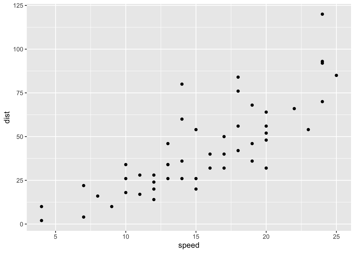
Then you’ll specify the mark (point here) that will take on the aesthetics (x or y position here, but color, size, shape are other examples), using geom_point()
Finally we might be interested in making some predictions; what is the expected value (mean) of y given some x (here stopping distance given some speed upon breaking) , using geom_smooth()