ggplot2 sublayer modularity

a brief and whimsical first-look behind the curtains of ggplot2’s layers

If you are a fan of ggplot2, you are probably also a fan of ‘layer’ functions geom_*() and stat_*().

Important clarification before we begin: Sometimes all the ggplot2 functions are referred to as ggplot2 ‘layers’, i.e. scales_*(), coord_*(), etc as in ‘build up your plot layer-by-layer’. *

But we are using the word in the narrower, sense used in the ggplot2 documentation.

Maybe you get giddy thinking about geom_bump(), geom_ridgeline(), or classic geom_histogram()?

Well-composed geom_*()s and stat_*()s (i.e. layer) make for more fluid analytic discovery.

But what elements constitute a layer function?

Let’s look at geom_bar() to get a feel for what layer composition means.

In this plot specification, geom_bar() counts the number of observations that are of each value of x (cut).

There are actually three main characters in every geom_() or stat_().

They are geom, stat, and position.

In geom_bar() the geom is fixed, but stat and position are adjustable. You can see that their defaults are "count" and "stack" in the function’s definition.

And instead of using convenient geom_bar(), we can use the more generic layer() function - which is actually used under the hood to define all geom_*() and stat_*() functions.

We can reproduce `geom_bar()`‘s behavior with layer(), but we must provide all three ’control operators’:layer(geom = "bar", stat = "count", position = "stack").

Or, equivalently, we can simply name the underlying ggproto objects, GeomBar and StatCount in our case, and the position function, position_stack() .

Reiteration: There are actually ‘control operators’ that define the geom_*() and stat_*() user-facing function. Geoms, Stats, and position_*().

You can refer to them indirectly by quoting their stem, layer(geom = "bar", stat = "count", position = "stack").

Or use the ggproto objects and position function directly, layer(geom = GeomBar, stat = StatCount, position = position_stack())

Focus: Lets look at one ‘control operator’, the Stat, more closely.

Stats themselves have a number of control elements.

It transforms plot input data before it is passed off to be rendered.

Stat’s computation is defined in the compute slots.

And in StatCount, compute is done group-wise, so compute_group() defines StatCount’s data transformation.

We can get a sense of StatCount$compute_group’s behavior by using on our data.

First, we use select() to make the data look as it would inside of the ggplot2 plotting environment — this mirrors the aes(x = cut) mapping declaration.

Then we see that the data is collapsed by x, and count and prop variables are produced.

We can think about StatCount’s job as doing some computation that the user might otherwise be responsible for.

We use StatCount$compute_group() to manually do this computation for us, in conjunction with StatIdentity (leaves data alone) in layer to show this work explicitly.

Key point: We might think Stat’s job as lightening the analyst’s load - doing computation that the user would otherwise need to do for before plotting.

One final question you might have is ’how exactly is the height of the bar, y, communicated to the ggplot2 system? Why does that just work?

This is managed by the default_aes specification for StatCount.

Because there is no variable mapped to y in our plot specification, y position defaults to after_stat(count), in other words the computed variable count that is available after the StatCount computation is done!

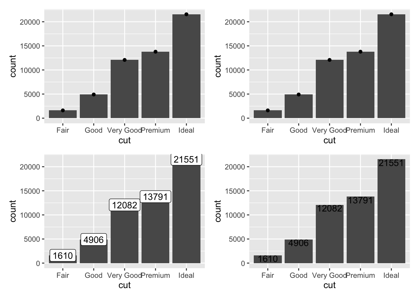
And it is good to do a little mix-and-match thinking to get a further feel for StatCount. Which of the following plots will have identical outputs?

Is this what you anticipated?

Above, we’ve had an outside-in look at some aspects of ‘sublayer modularity’.

To get an inside-out look — building up your own Stat from scratch — you might have a look at ‘easy geom recipes’ or by joining ggplot2 extenders club

library(ggplot2) 
ggplot(diamonds) + 
  aes(x = cut) + 
  geom_bar()

geom_bar

function (mapping = NULL, data = NULL, stat = "count", position = "stack", 
    ..., just = 0.5, na.rm = FALSE, orientation = NA, show.legend = NA, 
    inherit.aes = TRUE) 
{
    layer(data = data, mapping = mapping, stat = stat, geom = GeomBar, 
        position = position, show.legend = show.legend, inherit.aes = inherit.aes, 
        params = list2(just = just, na.rm = na.rm, orientation = orientation, 
            ...))
}
<bytecode: 0x7fe7c772e5b8>
<environment: namespace:ggplot2>

library(ggplot2) 
ggplot(diamonds) + 
  aes(x = cut) + 
  layer(geom = "bar", stat = "count", position = "stack")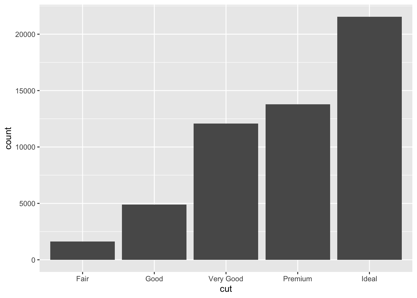

library(ggplot2) 
ggplot(diamonds) + 
  aes(x = cut) + 
  layer(geom = GeomBar, stat = StatCount, position = position_stack())

StatCount |> names()

[1] "default_aes"   "extra_params"  "super"         "compute_group"
[5] "required_aes"  "setup_params"  "dropped_aes"  

StatCount$compute_group

<ggproto method>
  <Wrapper function>
    function (...) 
compute_group(..., self = self)

  <Inner function (f)>
    function (self, data, scales, width = NULL, flipped_aes = FALSE) 
{
    data <- flip_data(data, flipped_aes)
    x <- data$x
    weight <- data$weight %||% rep(1, length(x))
    count <- as.vector(rowsum(weight, x, na.rm = TRUE))
    bars <- data_frame0(count = count, prop = count/sum(abs(count)), 
        x = sort(unique0(x)), width = width, flipped_aes = flipped_aes, 
        .size = length(count))
    flip_data(bars, flipped_aes)
}

library(dplyr)

diamonds |> 
  select(x = cut) |>
  StatCount$compute_group() 

  count       prop         x flipped_aes
1  1610 0.02984798      Fair       FALSE
2  4906 0.09095291      Good       FALSE
3 12082 0.22398962 Very Good       FALSE
4 13791 0.25567297   Premium       FALSE
5 21551 0.39953652     Ideal       FALSE

precomputation <- diamonds |> 
  select(x = cut) |>
  StatCount$compute_group()

precomputation |>
  ggplot() + 
  aes(x = x, y = count) + 
  layer(geom = GeomBar, 
        stat = StatIdentity, 
        position = position_stack())

StatCount$default_aes

Aesthetic mapping: 
* `x`      -> `after_stat(count)`
* `y`      -> `after_stat(count)`
* `weight` -> 1

ggplot(data = diamonds) + 
  aes(x = cut) + 
  layer(geom = GeomBar, 
        stat = StatCount, 
        position = position_stack())

p1 <- ggplot(data = diamonds) + 
  aes(x = cut) + 
  layer(geom = GeomBar, 
        stat = StatCount, 
        position = position_stack())

p2 <- p1 + geom_point(stat = StatCount)

p3 <- p1 + stat_count(geom = GeomPoint)

p4 <- p1 + geom_label(stat = StatCount, 
                      aes(label = after_stat(count)))

p5 <- p1 + stat_count(geom = GeomText, 
                      aes(label = after_stat(count)), 
                      vjust = 1)

library(patchwork)
p2+ p3 + p4 + p5