Recipe #1, `geom_medians() and geom_means()`

The Goal

In this first recipe, we’ll look at simple examples of defining a new geom_*() function, geom_medians() and geom_means().

Each geom_*() function (layer) is defined by three major elements: a Geom, a Stat, and a position. The simplest among these to create is a new Stat, so the ‘Easy recipes’ start with these. And while simple, Stats are also powerful because they allow you compute to be integrated into your plotting pipeline — that you would otherwise might need to do ‘manually’ before plotting.

Along with writing the geom_\*() function, we’ll write a stat_*() function, which is pretty typical for seasoned ggplot2 developers when writing Stats. It’s okay if you don’t typically write your plots with stat_*() functions – you can use just use the geom_*() functions if you like.

Note that in the ggplot2 extension context, the word ‘layer’ only refers to geom_*(), stat_*(), and annotate() functions. These all use the layer() function internally – a function that requires — you guessed it — a Geom, a Stat, and a position!

Let’s get started! Our objective in this first ‘recipe’ is to be able to compose the following plot with a new geom_means() function that we will create.

ggplot(data = penguins) + 
  aes(x = bill_depth_mm,
      y = bill_length_mm) + 
  geom_point() + 
  geom_means(size = 8, color = "red") # new function!

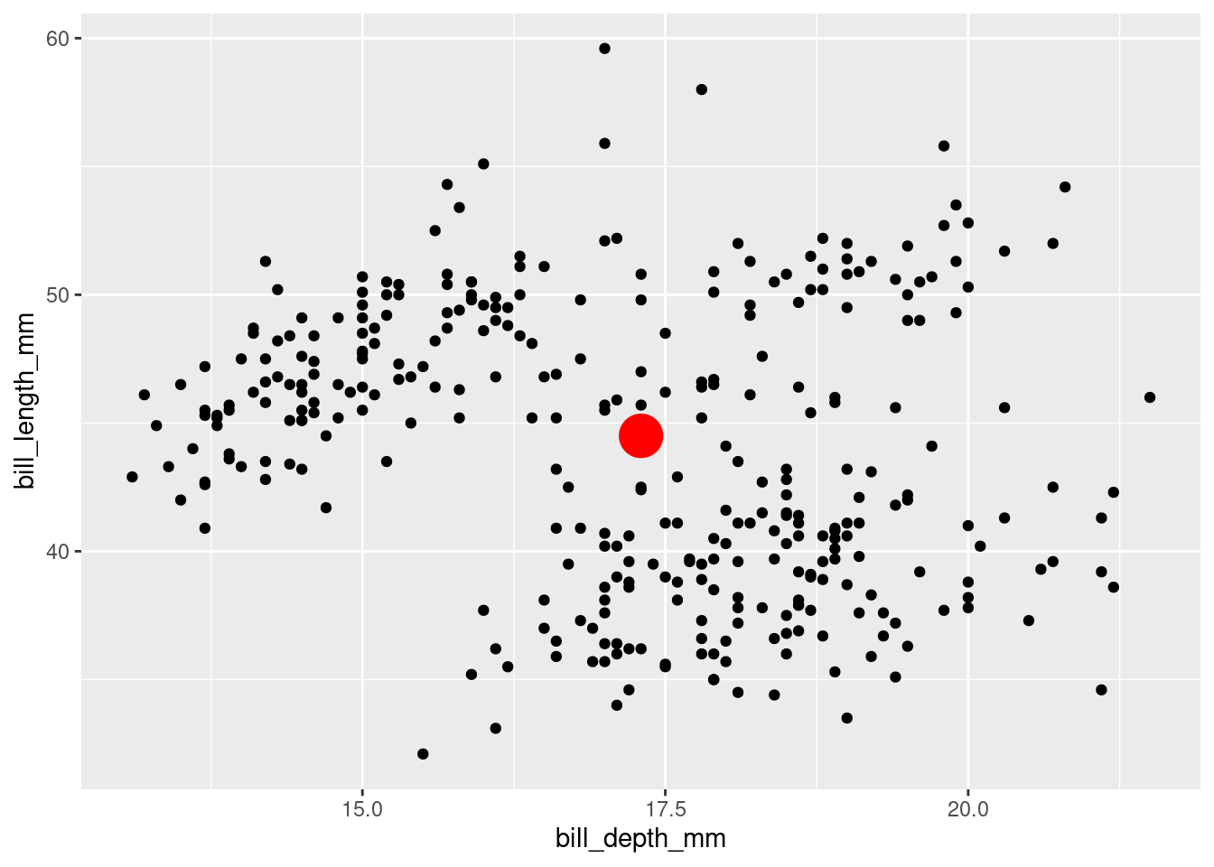
In this exercise, we’ll demonstrate how to define the new extension function geom_medians() to add a point at the medians x and y. Then you’ll be prompted to define geom_means() based on what you’ve learned.

Step 00: Loading packages and prepping data

library(tidyverse)
library(palmerpenguins)
glimpse(penguins)

Rows: 344
Columns: 8
$ species           <fct> Adelie, Adelie, Adelie, Adelie, Adelie, Adelie, Adel…
$ island            <fct> Torgersen, Torgersen, Torgersen, Torgersen, Torgerse…
$ bill_length_mm    <dbl> 39.1, 39.5, 40.3, NA, 36.7, 39.3, 38.9, 39.2, 34.1, …
$ bill_depth_mm     <dbl> 18.7, 17.4, 18.0, NA, 19.3, 20.6, 17.8, 19.6, 18.1, …
$ flipper_length_mm <int> 181, 186, 195, NA, 193, 190, 181, 195, 193, 190, 186…
$ body_mass_g       <int> 3750, 3800, 3250, NA, 3450, 3650, 3625, 4675, 3475, …
$ sex               <fct> male, female, female, NA, female, male, female, male…
$ year              <int> 2007, 2007, 2007, 2007, 2007, 2007, 2007, 2007, 2007…

Step 0: use base ggplot2 to get the job done

It’s a good idea to get things done without Stat extension first, just using ‘base’ ggplot2. The computational moves you make here can serve a reference for building our extension function.

# Compute.
penguins_medians <- penguins |> 
  summarize(bill_length_mm_median = median(bill_length_mm, na.rm = T),
            bill_depth_mm_median = median(bill_depth_mm, na.rm = T))

# Plot.
penguins |> 
  ggplot() + 
  aes(x = bill_depth_mm, y = bill_length_mm) + 
  geom_point() + 
  geom_point(data = penguins_medians,
             aes(x = bill_depth_mm_median,
                 y = bill_length_mm_median),
             size = 8, color = "red") + 
  labs(title = "Created with base ggplot2")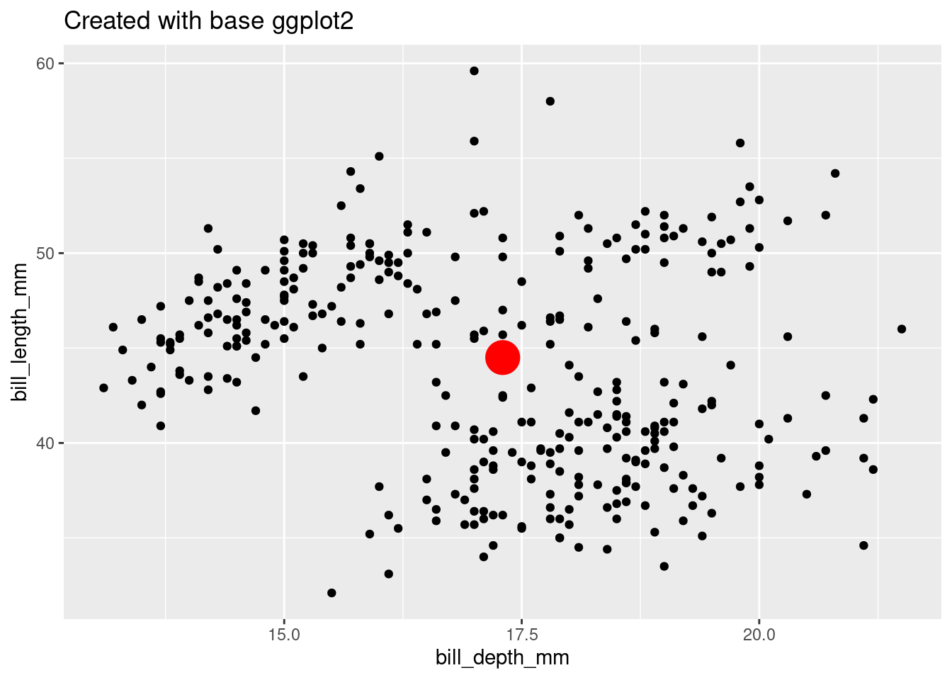

Pro tip. Use layer_data() to inspect ggplot's internal data …

Use ggplot2::layer_data() to inspect the render-ready data internal in the plot. Your Stat will help prep data to look something like this.

layer_data(plot = last_plot(), 
           i = 2) # layer 2, the computed means, is of interest

     x     y PANEL group shape colour size fill alpha stroke
1 17.3 44.45     1    -1    19    red    8   NA    NA    0.5

Step 1: Define compute. Test.

Now you are ready to begin building your extension function. The first step is to define the compute that should be done under-the-hood when your function is used. We’ll define this in a function called compute_group_medians(). The data input will look similar to the plot data. You will also need to include a scales argument, which ggplot2 uses internally.

Define compute.

# Define compute.
compute_group_medians <- function(data, scales){ 
  data |> 
    summarize(x = median(x, na.rm = T),
              y = median(y, na.rm = T))
}

You may have noticed …

… the scales argument in the compute definition, which is used internally in ggplot2. While it won’t be used in your test (up next), you do need so that the computation will work in the ggplot2 setting.
… that the compute function can only be used with data with variables x and y. These aesthetic variables names, relevant for building the plot, are generally not found in the raw data inputs for plot.

Test compute.

# Test compute. 
penguins |>
  select(x = bill_depth_mm,  
         y = bill_length_mm) |>  
  compute_group_medians()

# A tibble: 1 × 2
      x     y
  <dbl> <dbl>
1  17.3  44.4

You may have noticed …

… that we prepare the data to have columns with names x and y before testing. Computation will fail if variables x and y are not present given the function’s definition. In a plotting setting, columns are renamed by mapping aesthetics, e.g. aes(x = bill_depth, y = bill_length).

Step 2: Define new Stat. Test.

Next, we use the ggplot2::ggproto function which allows you to define a new Stat object - which will let us do computation under the hood while building our plot.

Define Stat.

StatMedians <- 
  ggplot2::ggproto(`_class` = "StatMedians",
                   `_inherit` = ggplot2::Stat,
                   compute_group = compute_group_medians,
                   required_aes = c("x", "y"))

You may have noticed…

… that the naming convention for the ggproto object is written in CamelCase. The new class should also be named the same, i.e. "StatMedians".
… that we inherit from the ‘Stat’ class. In fact, your ggproto object is a subclass – you are inheriting class properties from ggplot2::Stat.
… that the compute_group_medians function is used to define our Stat’s compute_group element. This means that data will be transformed group-wise by our compute definition – i.e. by categories if a categorical variable is mapped.
… that setting required_aes to x and y reflects the compute functions requirements Specifying required_aes in your Stat can improve your user interface. Standard ggplot2 error messages will issue if required aes are not specified, e.g. “stat_medians() requires the following missing aesthetics: x.”

Test Stat.

You can test out your Stat using them in ggplot2 geom_*() functions.

penguins |> 
  ggplot() + 
  aes(x = bill_depth_mm,
      y = bill_length_mm) + 
  geom_point() + 
  geom_point(stat = StatMedians, size = 7) + 
  labs(title = "Testing StatMedians")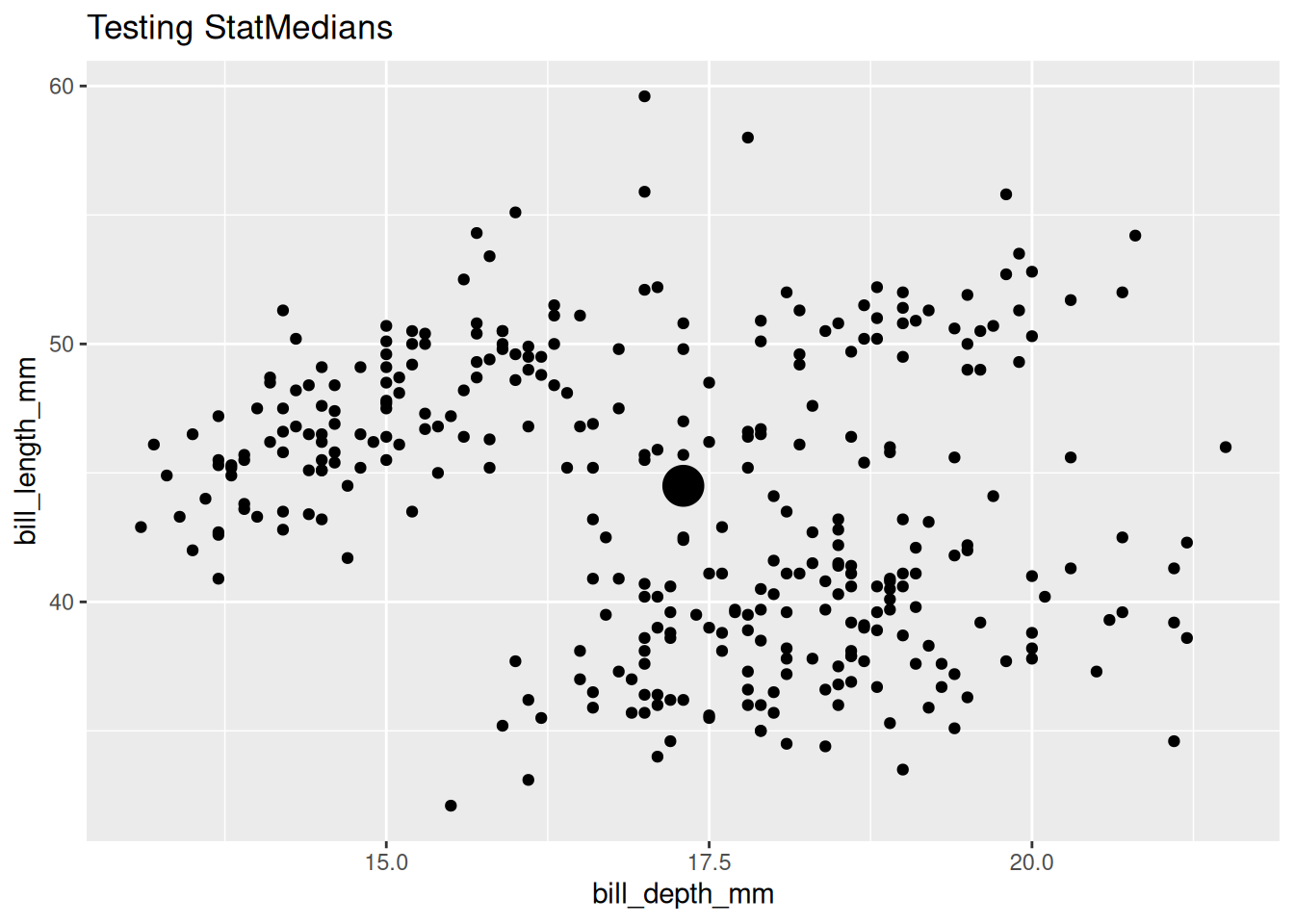

You may have noticed …

… that we don’t use "medians" as the stat argument. But you could! If you prefer, you could write geom_point(stat = "medians", size = 7) which will direct to your new StatMedians under the hood.

Test Stat group-wise behavior

Test group-wise behavior by using a discrete variable with an group-triggering aesthetic like color, fill, or group, or by faceting.

last_plot() + 
  aes(color = species)

Pro tip: Think about an early exit (don’t define a user-facing function) …

You might be thinking, what we’ve done would already be pretty useful to me. Can I just use my Stat as-is within geom_*() functions?

The short answer is ‘yes’! If you just want to use the Stat yourself locally in a script, there might not be much reason to go on to Step 3, user-facing functions. But if you have a wider audience in mind, i.e. internal to organization or open sourcing in a package, probably a more succinct expression of what functionality you deliver will be useful - i.e. write the user-facing functions.

Pro tip: consider using layer() function to test instead of geom_*(stat = StatNew)

Instead of using a geom_*() function, you might prefer to use the layer() function in your testing step. Occasionally, you must to go this route; for example, geom_vline() contain no stat argument, but you can use the GeomVline in layer(). If you are teaching this content, using layer() may help you better connect this step with the next, defining the user-facing functions.

A test of StatMedians using this method follows. You can see it is a little more verbose, as there is no default for the position argument, and setting the size must be handled with a little more care.

penguins |> 
  ggplot() + 
  aes(x = bill_depth_mm,
      y = bill_length_mm) + 
  geom_point() + 
  layer(geom = GeomPoint, 
        stat = StatMedians, 
        position = "identity", 
        params = list(size = 7)) + 
  labs(title = "Testing StatMedians with layer() function")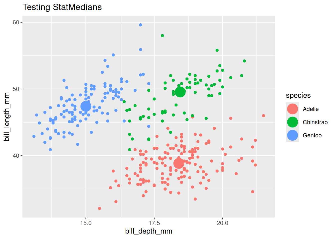

Step 3: Define user-facing functions. Test.

In this next section, we define user-facing functions. Doing so is a bit of a mouthful, but see the ‘Pro tip: Use geom_point definition as a template in this step …’ that follows.

Define stat_() and geom_() functions.

stat_medians <- function (mapping = NULL, data = NULL,
                          geom = "point", position = "identity",
                          ..., na.rm = FALSE, 
                          show.legend = NA, inherit.aes = TRUE) 
{
    layer(mapping = mapping, data = data, 
          geom = geom, stat = StatMedians, 
          position = position, show.legend = show.legend, 
          inherit.aes = inherit.aes, 
        params = rlang::list2(na.rm = na.rm, ...))
}

You may have noticed that …

… the stat_*() function name derives from the Stat object’s name, but is snake case. Given naming conventions, a StatBigCircle-based stat_*() function, should be named stat_big_circle().
… StatMedians defines the new layer function and cannot be replaced by the user StatMedians and the computation that defines it will be in effect before the layer is rendered.
… "point" refers to the object GeomPoint and defines the layer’s geom unless otherwise specified.

Pro tip. 🎉 Use make_constructor() to write the scaffolding code for you upon the next ggplot2 release.

stat_medians <- make_constructor(StatMedians, geom = "point")

Define geom_*() function

Because users are more accustom to using layers that have the geom_ prefix, you might also define a geom_ function with identical properties as the stat_ via aliasing.

‘Most ggplot2 users are accustomed to adding geoms, not stats, when building up a plot.’ ggplot2: Elegant Graphics for Data Analysis.

geom_medians <- stat_medians

Be aware that verbatim aliasing as shown above is a bit of a shortcut, and a tad unconventional.

It is more conventional write out scaffolding code, nearly identical to the stat_*() definition, but has the geom fixed and the stat flexible.

But soon we can use make_constructor() in the next ggplot2 release, just about as easy as aliasing and which will deliver the fixed-geom, flexible-stat convention in what follows:

geom_medians <- make_constructor(GeomPoint, stat = "medians")

Test/Enjoy your user-facing functions

Test geom_medians()

## Test user-facing.
penguins |>
  ggplot() +
  aes(x = bill_depth_mm, y = bill_length_mm) +
  geom_point() +
  geom_medians(size = 8)  + 
  labs(title = "Testing geom_medians()")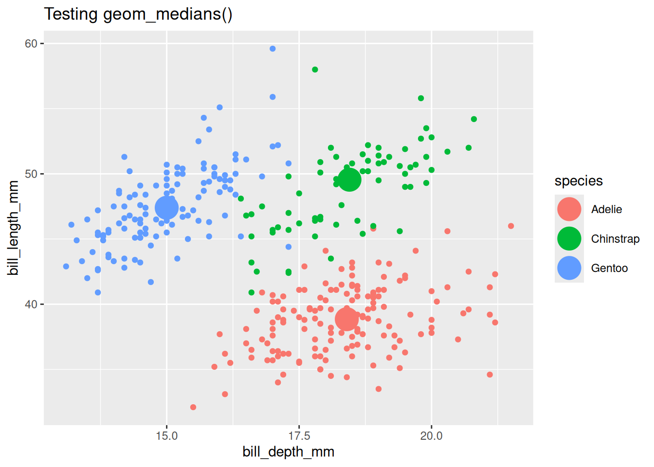

Test group-wise behavior

last_plot() + 
  aes(color = species)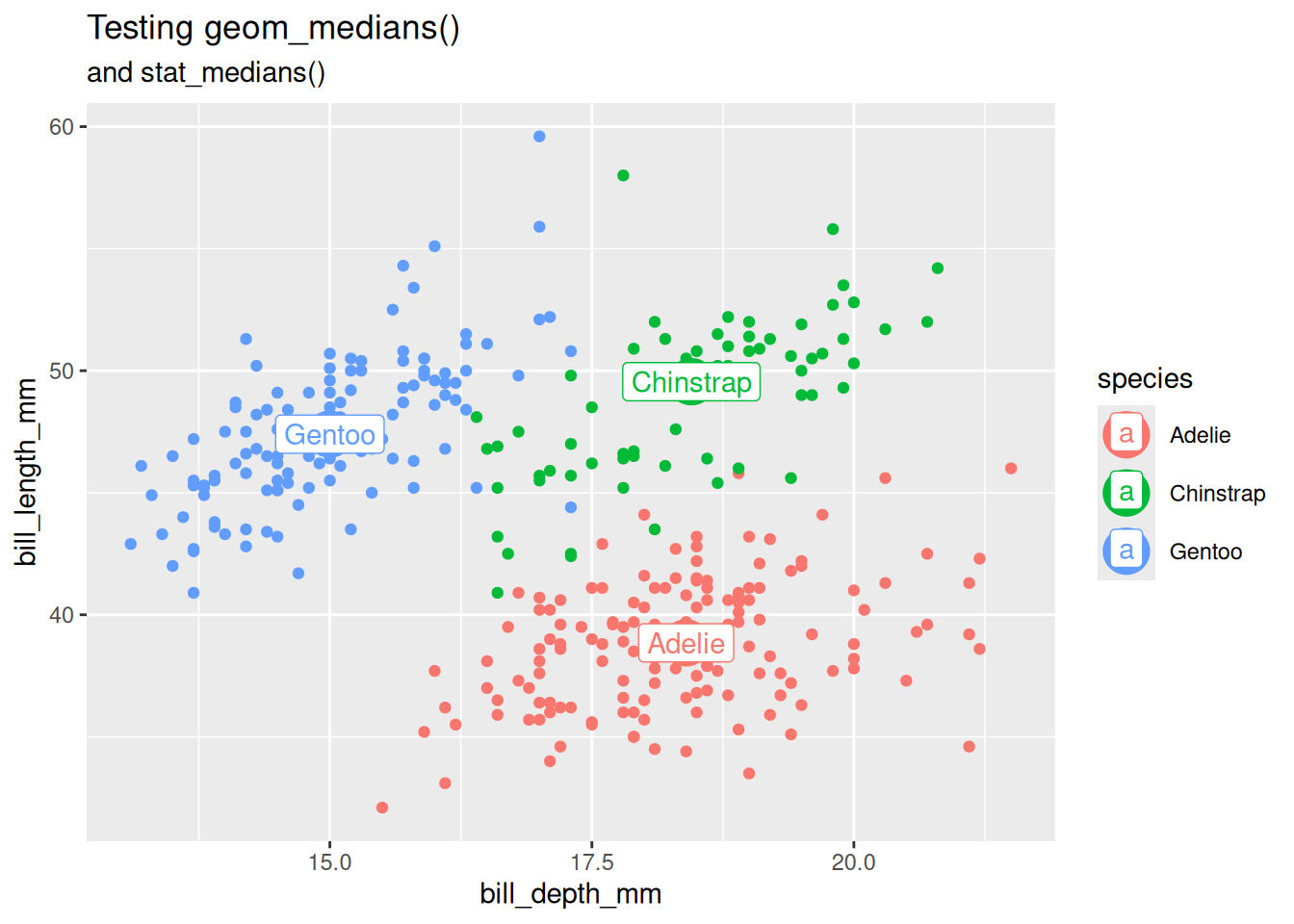

Test stat_*() function with another Geom.

last_plot() + 
  stat_medians(geom = "label", aes(label = species))  + 
  labs(subtitle = "and stat_medians()")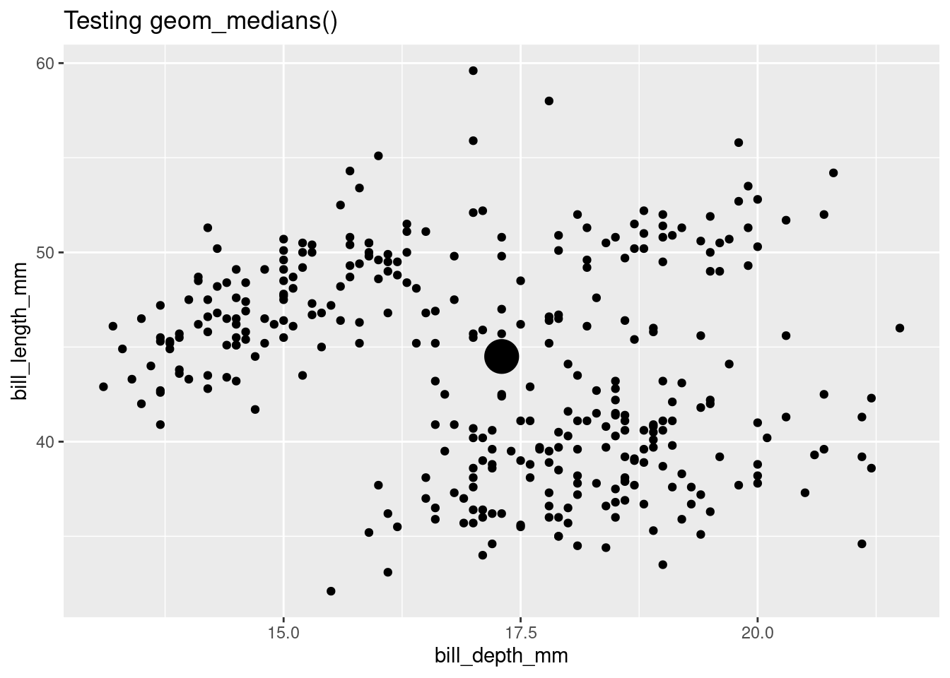

Done! Time for a review.

Here is a quick review of the functions and ggproto objects we’ve covered, dropping tests and discussion.

Review

library(tidyverse)

# Step 1. Define compute
compute_group_medians <- function(data, scales){
  
  data |>
    summarise(x = median(x), y = median(y))
  
}

# Step 2. Define Stat
StatMedians = ggproto(`_class` = "StatMedians",
                      `_inherit` = Stat,
                      required_aes = c("x", "y"),
                      compute_group = compute_group_medians)

# Step 3. Define user-facing functions (user friendly, geom_*() function only shown here)

## use geom_point's definition as a model to follow geom_* conventions: geom is fixed, stat is flexible
stat_medians <- function(mapping = NULL, data = NULL, 
                         geom = "point", position = "identity", 
                         ..., show.legend = NA, inherit.aes = TRUE) 
{
    layer(data = data, mapping = mapping, stat = StatMedians, 
        geom = geom, position = position, show.legend = show.legend, 
        inherit.aes = inherit.aes, params = rlang::list2(na.rm = FALSE, 
            ...))
}

# stat_medians
geom_medians <- stat_medians

Your Turn: write `geom_means()`

Using the geom_medians Recipe #1 as a reference, try to create a geom_means() function that draws a point at the means of x and y. You may also write convenience geom_*() functions.

Step 00: load libraries, data

Step 0: Use base ggplot2 to get the job done

Step 1: Write compute function. Test.

Step 2: Write Stat.

Step 3: Write user-facing functions

Next up: Recipe 2 `geom_id()`

How would you write the function which annotates coordinates (x,y) for data points on a scatterplot? Go to Recipe 2.

Pro tip: check out ggplot2::stat_manual() for one-off group-wise compute in the next ggplot2 release or statexpress::qstat() for a quick stat short-cut in extension explorations.

Examples follow:

## Consider statexpress::qstat_*() functions for more 
## flexibility and exploratory extension work 
mean_fun <- function(data, scales){
  
  data |>
    summarize(x = mean(x, na.rm = T),
              y = mean(y, na.rm = T))
}

library(statexpress)
ggplot(penguins) + 
  aes(x = bill_depth_mm,
      y = bill_length_mm) + 
  geom_point() + 
  geom_point(stat = qstat(mean_fun),
             size = 8)
#--------------------------------------------------

## option 2, use geom_point(stat = "manual")
means_fun2 <- function(data){
  
  data |>
    summarize(x = mean(x, na.rm = T),
              y = mean(y, na.rm = T))
  
}

### usage A (geom )
ggplot(penguins) + 
  aes(x = bill_depth_mm,
      y = bill_length_mm) + 
  geom_point() + 
  geom_point(stat = "manual",
             fun = means_fun2, 
             size = 8)

### usage B (geom )
ggplot(penguins) + 
  aes(x = bill_depth_mm,
      y = bill_length_mm) + 
  stat_manual(size = 8, # geom default is "point"
              fun = means_fun2)

The Goal

Step 00: Loading packages and prepping data

Step 0: use base ggplot2 to get the job done

Step 1: Define compute. Test.

Define compute.

Test compute.

Step 2: Define new Stat. Test.

Define Stat.

Test Stat.

Test Stat group-wise behavior

Step 3: Define user-facing functions. Test.

Define stat_*() and geom_*() functions.

Define geom_*() function

Test/Enjoy your user-facing functions

Test geom_medians()

Test group-wise behavior

Test stat_*() function with another Geom.

Done! Time for a review.

Your Turn: write geom_means()

Step 00: load libraries, data

Step 0: Use base ggplot2 to get the job done

Step 1: Write compute function. Test.

Step 2: Write Stat.

Step 3: Write user-facing functions

Next up: Recipe 2 geom_id()

Define stat_() and geom_() functions.

Your Turn: write `geom_means()`

Next up: Recipe 2 `geom_id()`