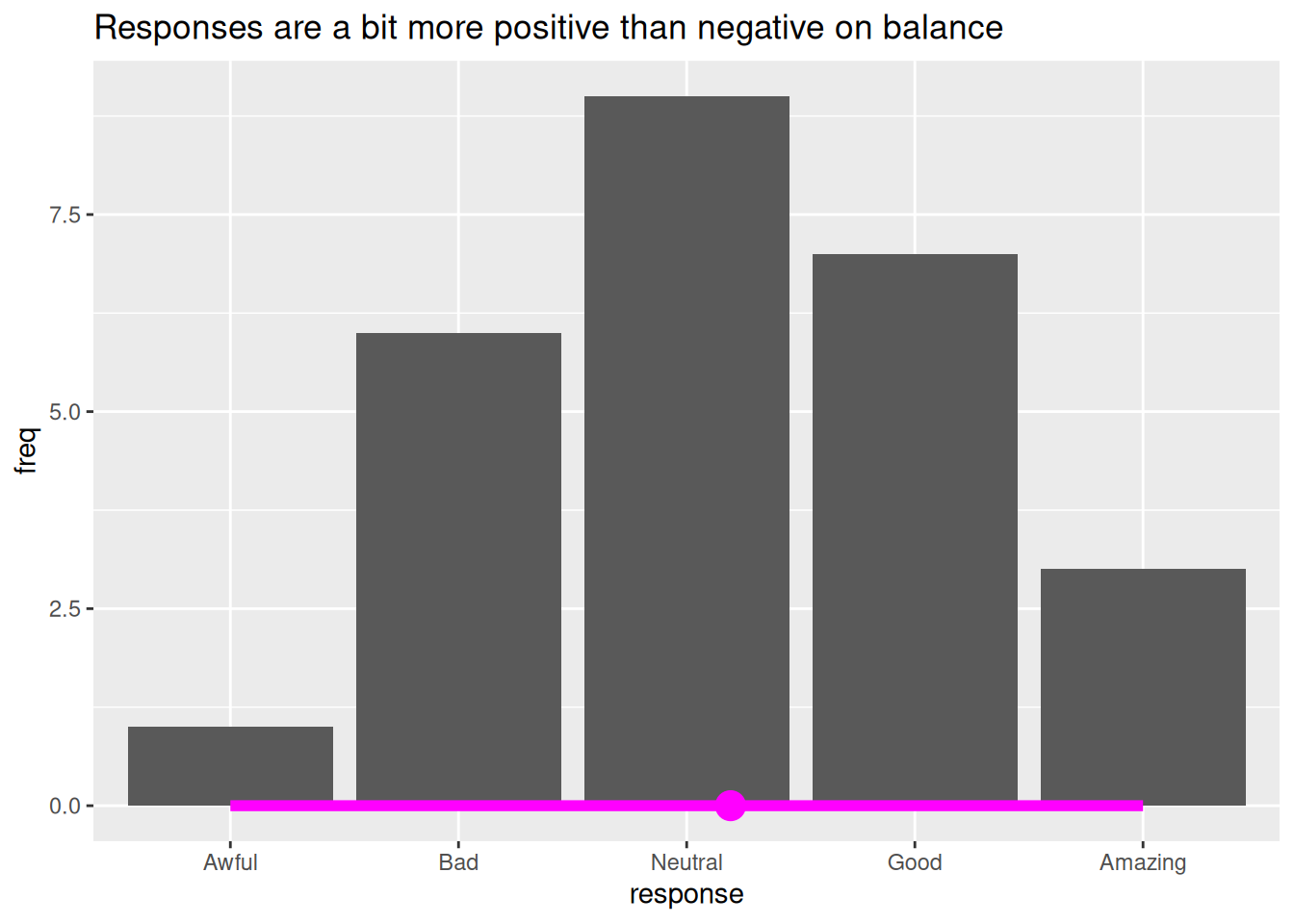
survey_df <- data.frame(response =
             c("Awful", "Bad",
                        "Neutral",
                        "Good",
                        "Amazing") |>
                          fct_inorder(ordered = T),
                         freq = c(1, 6, 9, 7, 3))

ggplot(data = survey_df) +
  aes(x = response,
      y = freq) +
  geom_col() +
  geom_support(color = "magenta",
               size = 2) +
  geom_bal_point(color = "magenta",
size = 7)Recipe 3: geom_bal_point() and geom_support()
In the first two of recipes, you defined compute that would work group-wise. In recipe #2 we briefly we contrasted a panel-wise computation specification with our group-wise computation (see StatIndexPanel). We saw that when introducing a categorical variable using StatIndexPanel, indices were computed across the groups, instead of within groups – the behavior for StatIndex.
In this recipe, we’ll use panel-wise computation throughout to look at the ‘balance’ of the frequency of discrete ordinal variables. Panel-wise compute is needed because of the discrete variable mapping, i.e. aes(x = response). So that the data isn’t broken up by category (unique responses), we define compute_panel instead of compute_group.
Our goal is to be able to write the following code, producing the plot that follows.
Let’s get started!
Step 0: use base ggplot2 to get the job done
It’s a good idea to look at how you’d get things done without extension first, just using ‘base’ ggplot2. Here, we’ll plot the frequencies of some ordered responses (A to E), and look at the ‘balance’ based on their numeric values.
library(tidyverse)
survey_df <- data.frame(response =
                          c("Awful",
                        "Bad",
                        "Neutral",
                        "Good",
                        "Amazing") |>
                          fct_inorder(ordered = T),
                         freq = c(1, 6, 9, 7, 3))

balancing_point_df <- survey_df |>
  summarize(x = sum(as.numeric(response) * freq) /
              sum(freq)) |>
  mutate(y = 0)

ggplot(survey_df) +
  aes(x = response,
      y = freq) +
  geom_col() +
  geom_point(data = balancing_point_df,
             aes(x = x, y = y),
             size = 5, color = "magenta")
Step 1: Define compute. Test.
Now you are ready to begin building your extension function. The first step is to define the compute that should be done under-the-hood when your function is used. We’ll define this in a function called compute_panel_bal_point(). You will also need to include a scales argument, which ggplot2 uses internally. Because the x scale is converted to numeric early on in ggplot2 plot build - the compute is even simpler - you don’t need to convert your x variable to numeric as was required in Step 0!
compute_panel_bal_point <- function(data, scales){

  data |>
  summarize(x = sum(x * y) / sum(y)) |>
  mutate(y = 0)

}
NoteYou may have noticed …
… the
scalesargument in the compute definition, which is used internally in ggplot2. While it won’t be used in your test (up next), you do need so that the computation will work in the ggplot2 setting.… that the compute function can only be used with data with variables
xAesthetic variables names, relevant for building the plot, are generally not found in the raw data inputs for plot.
Test compute.
## Test compute.
survey_df |>
  mutate(response = response |> as.numeric()) |>
  select(x = response,
         y = freq) |>
  compute_panel_bal_point()
x y
1 3.192308 0
NoteYou may have noticed …
… that we prepare the data to have columns with names x and y before testing compute_panel_bal_point. Computation will fail if the names x and y are not present given our function definition. Internally in a plot, columns are named based on aesthetic mapping, e.g. aes(x = response, y = freq).
Step 2: Define new Stat. Test.
Next, we use the ggplot2::ggproto function which allows you to define a new Stat object - which will let us do computation under the hood while building our plot.
Define Stat.
StatBalPoint <- ggplot2::ggproto(`_class` = "StatBalPoint",
                                  `_inherit` = ggplot2::Stat,
                                  required_aes = c("x", "y"),
                                  compute_panel = compute_panel_bal_point)
NoteYou may have noticed …
… that the naming convention for the ggproto object is CamelCase. The new class should also be named the same, i.e.
"StatLmFitted".… that we inherit from the ‘Stat’ class. In fact, your ggproto object is a subclass and you aren’t fully defining it. You simplify the definition by inheriting class properties from ggplot2::Stat.
that the compute_panel_lm_cat function is used to define our Stat’s compute_panel element. This means that data will be transformed by our compute definition – group-wise if groups are specified.
that setting
required_aesto ‘x’, ‘y’, and ‘cat’ is consistent with compute requirements The compute assumes data to be a dataframe with columns x and y. If you data doesn’t have x, y, and cat your compute will fail. Specifyingrequired_aesin your Stat can improve your user interface because standard ggplot2 error messages will issue when required aes are not specified, e.g. ‘stat_lm_cat()requires the following missing aesthetics: x.’
Test Stat.
You can test out your Stat using them in ggplot2 geom_*() functions.
survey_df |>
  ggplot() +
  aes(x = response,
      y = freq) +
  geom_col() +
  geom_point(stat = StatBalPoint,
             color = "magenta",
             size = 7) +
  labs(title = "Testing StatBalPoint")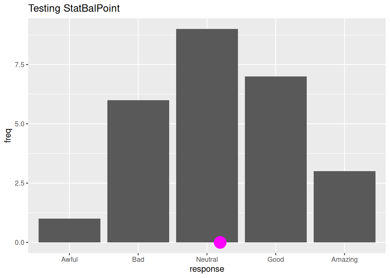
NoteYou may have noticed …
that we don’t use "bal_point" as the stat argument, which - but you could! StatBalPoint would be retrieved under the hood.
TipPro tip: Think about an early exit (don’t define use facing functions) …
You might be thinking, what we’ve done would already be pretty useful to me. Can I just use my Stat as-is within geom_*() functions?
The short answer is ‘yes’! If you just want to use the Stat yourself locally in a script, there might not be much reason to go on to Step 3, user-facing functions. But if you have a wider audience in mind, i.e. internal to organization or open sourcing in a package, probably a more succinct expression of what functionality you deliver will be useful - i.e. write the user-facing functions.
TipPro tip: consider using
layer() function to test instead of geom_*(stat = StatNew)
Instead of using a geom_*() function, you might prefer to use the layer() function in your testing step. Occasionally, it’s necessary to go this route; for example, geom_vline() contain no stat argument, but you can use the GeomVline in layer(). If you are teaching this content, using layer() may help you better connect this step with the next, defining the user-facing functions.
A test of StatBalPoint using this method follows. You can see it is a little more verbose, as there is no default for the position argument, and setting the size must be handled with a little more care.
survey_df |>
  ggplot() +
  aes(x = response,
      y = freq) +
  geom_col() +
  layer(geom = GeomPoint,
        stat = StatBalPoint,
        position = "identity",
        params = list(color = "magenta")) +
  labs(title = "Testing StatBalPoint with layer() function")
Step 3: Define user-facing functions. Test.
In this next section, we define user-facing functions. Doing so is a bit of a mouthful, but see the ‘Pro tip: Use stat_identity definition as a template in this step …’ that follows.
stat_bal_point <- function(mapping = NULL, data = NULL, geom = "point", position = "identity",
    ..., show.legend = NA, inherit.aes = TRUE) {
    layer(data = data, mapping = mapping, stat = StatBalPoint,
        geom = geom, position = position, show.legend = show.legend,
        inherit.aes = inherit.aes, params = list(na.rm = FALSE,
            ...))
}
NoteYou may have noticed…
… that the
stat_*()function name derives from the Stat objects’s name, but is snake case. So if I wanted a StatBigCircle-based stat_*() function, I’d create stat_big_circle().… that
StatBalPointis used to define the new layer function, so the computation that defines it, which is to summarize to medians, will be in play before the layer is rendered.… that
"point"is specified as the default for the geom argument in the function. This means that theggplot2::GeomPointwill be used in the layer unless otherwise specified by the user.
TipPro tip. 🎉 Use
make_constructor from the next ggplot2 release to write this scaffolding code for you!
stat_bal_point <- make_constructor(StatBalPoint, geom = "point")Define geom_*() function
Because users are more accustom to using layers that have the geom prefix, you might also define geom with similar properties.
geom_bal_point <- make_constructor(GeomPoint, stat = "bal_point")Test/Enjoy functions
survey_df |>
  ggplot() +
  aes(x = response,
      y = freq) +
  geom_col() +
  geom_bal_point(color = "magenta",
                 size = 7)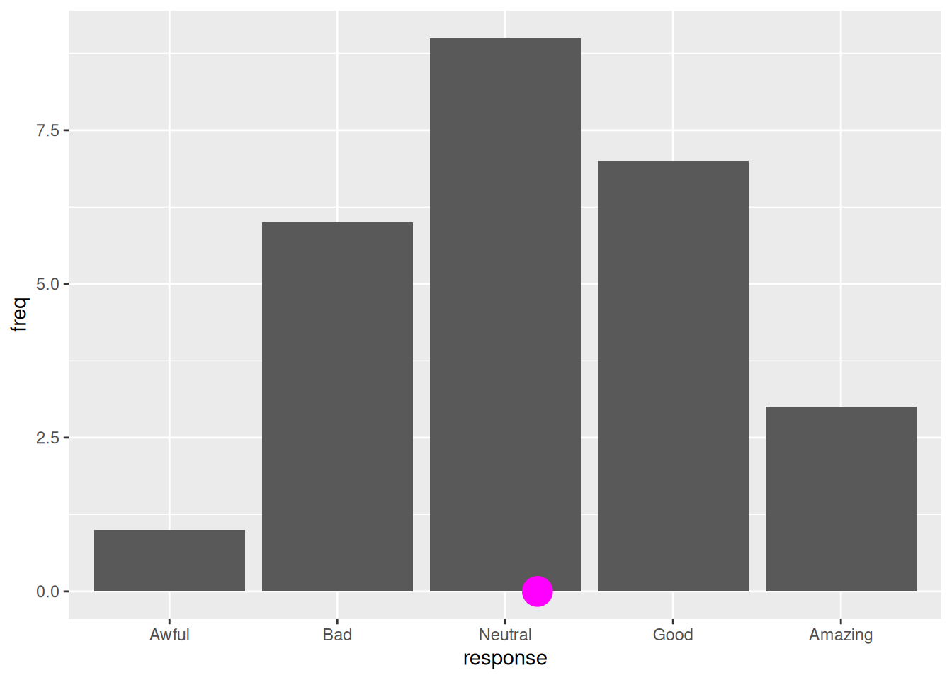
Done! Time for a review.
Here is a quick review of the functions and ggproto objects we’ve covered, dropping tests and discussion.
NoteReview
library(tidyverse)

# Step 1. Define compute
compute_panel_bal_point <- function(data, scales){

  data |>
    summarise(x = (x*y)/sum(y)) |>
    mutate(y = 0)

}


# Step 2. Define Stat
StatBalPoint = ggproto(`_class` = "StatBalPoint",
                      `_inherit` = Stat,
                      required_aes = c("x", "y"),
                      compute_group = compute_panel_bal_point)

# Step 3. Define user-facing functions

## define stat_*()
stat_bal_point <- make_constructor(StatBalPoint, geom = "point")


## define geom_*()
geom_bal_point <- make_constructor(GeomPoint, stat = "bal_point")
Your Turn: Write geom_support()
Using the geom_bal_point Recipe #3 as a reference, try to create a stat_support() and convenience geom_support() that draws a segment from the minimum of x to the max of x along y = 0. This might complement the geom_bal_point(), being the support upon which the data bars sit and the logical limits for the balancing point.
Hint: consider what aesthetics are required for segments. We’ll give you Step 0 this time…
Step 0: use base ggplot2 to get the job done
Step 1: Write compute function. Test.
Step 2: Write Stat.
Step 3: Write user-facing functions.
Next up, Recipe 4: geom_lm_cat()
How would you write the function draws residuals based on a linear model fit that contains a categorical variable, lm(y ~ x + cat)? Go to Recipe 4.