Recipe 3: geom_residuals()

Author

Gina Reynolds, Morgan Brown

Published

January 3, 2022

The Goal

Welcome to ‘Easy geom recipes’ Recipe #3: creating geom_fitted and geom_residuals.

Creating a new geom_*() or stat_*() function is often motivated when plotting would require pre-computation otherwise. By using Stat extension, you can define computation to be performed within the plotting pipeline, as in the code that follows:

Example recipe #3: `geom_fitted()`

Step 0: use base ggplot2 to get the job done

It’s a good idea to look at how you’d get things done without Stat extension first, just using ‘base’ ggplot2. The computational moves you make here can serve a reference for building our extension function.

library(tidyverse)

── Attaching core tidyverse packages ──────────────────────── tidyverse 2.0.0 ──
✔ dplyr     1.1.4     ✔ readr     2.1.5
✔ forcats   1.0.0     ✔ stringr   1.5.1
✔ ggplot2   3.5.2     ✔ tibble    3.2.1
✔ lubridate 1.9.4     ✔ tidyr     1.3.1
✔ purrr     1.0.4     
── Conflicts ────────────────────────────────────────── tidyverse_conflicts() ──
✖ dplyr::filter() masks stats::filter()
✖ dplyr::lag()    masks stats::lag()
ℹ Use the conflicted package (<http://conflicted.r-lib.org/>) to force all conflicts to become errors

penguins <- remove_missing(palmerpenguins::penguins)

Warning: Removed 11 rows containing missing values or values outside the scale
range.

model <- lm(formula = bill_length_mm ~ bill_depth_mm, 
            data = penguins) 

penguins_w_fitted <- penguins %>% 
  mutate(fitted = model$fitted.values)

penguins %>% 
  ggplot() + 
  aes(x = bill_depth_mm, y = bill_length_mm) +
  geom_point() + 
  geom_smooth(method = "lm", se = F) + 
  geom_point(data = penguins_w_fitted,
             aes(y = fitted),
             color = "blue")

`geom_smooth()` using formula = 'y ~ x'

Pro tip. Use layer_data() to inspect ggplot's internal data …

Use ggplot2::layer_data() to inspect the render-ready data internal in the plot. Your Stat will help prep data to look something like this.

layer_data(plot = last_plot(), 
           i = 2) # the fitted y (not the raw data y) is of interest

`geom_smooth()` using formula = 'y ~ x'

          x        y flipped_aes PANEL group  colour   fill linewidth linetype
1  13.10000 46.57360       FALSE     1    -1 #3366FF grey60         1        1
2  13.20633 46.50609       FALSE     1    -1 #3366FF grey60         1        1
3  13.31266 46.43858       FALSE     1    -1 #3366FF grey60         1        1
4  13.41899 46.37107       FALSE     1    -1 #3366FF grey60         1        1
5  13.52532 46.30356       FALSE     1    -1 #3366FF grey60         1        1
6  13.63165 46.23605       FALSE     1    -1 #3366FF grey60         1        1
7  13.73797 46.16854       FALSE     1    -1 #3366FF grey60         1        1
8  13.84430 46.10103       FALSE     1    -1 #3366FF grey60         1        1
9  13.95063 46.03353       FALSE     1    -1 #3366FF grey60         1        1
10 14.05696 45.96602       FALSE     1    -1 #3366FF grey60         1        1
11 14.16329 45.89851       FALSE     1    -1 #3366FF grey60         1        1
12 14.26962 45.83100       FALSE     1    -1 #3366FF grey60         1        1
13 14.37595 45.76349       FALSE     1    -1 #3366FF grey60         1        1
14 14.48228 45.69598       FALSE     1    -1 #3366FF grey60         1        1
15 14.58861 45.62847       FALSE     1    -1 #3366FF grey60         1        1
16 14.69494 45.56096       FALSE     1    -1 #3366FF grey60         1        1
17 14.80127 45.49345       FALSE     1    -1 #3366FF grey60         1        1
18 14.90759 45.42595       FALSE     1    -1 #3366FF grey60         1        1
19 15.01392 45.35844       FALSE     1    -1 #3366FF grey60         1        1
20 15.12025 45.29093       FALSE     1    -1 #3366FF grey60         1        1
21 15.22658 45.22342       FALSE     1    -1 #3366FF grey60         1        1
22 15.33291 45.15591       FALSE     1    -1 #3366FF grey60         1        1
23 15.43924 45.08840       FALSE     1    -1 #3366FF grey60         1        1
24 15.54557 45.02089       FALSE     1    -1 #3366FF grey60         1        1
25 15.65190 44.95338       FALSE     1    -1 #3366FF grey60         1        1
26 15.75823 44.88587       FALSE     1    -1 #3366FF grey60         1        1
27 15.86456 44.81837       FALSE     1    -1 #3366FF grey60         1        1
28 15.97089 44.75086       FALSE     1    -1 #3366FF grey60         1        1
29 16.07722 44.68335       FALSE     1    -1 #3366FF grey60         1        1
30 16.18354 44.61584       FALSE     1    -1 #3366FF grey60         1        1
31 16.28987 44.54833       FALSE     1    -1 #3366FF grey60         1        1
32 16.39620 44.48082       FALSE     1    -1 #3366FF grey60         1        1
33 16.50253 44.41331       FALSE     1    -1 #3366FF grey60         1        1
34 16.60886 44.34580       FALSE     1    -1 #3366FF grey60         1        1
35 16.71519 44.27829       FALSE     1    -1 #3366FF grey60         1        1
36 16.82152 44.21078       FALSE     1    -1 #3366FF grey60         1        1
37 16.92785 44.14328       FALSE     1    -1 #3366FF grey60         1        1
38 17.03418 44.07577       FALSE     1    -1 #3366FF grey60         1        1
39 17.14051 44.00826       FALSE     1    -1 #3366FF grey60         1        1
40 17.24684 43.94075       FALSE     1    -1 #3366FF grey60         1        1
41 17.35316 43.87324       FALSE     1    -1 #3366FF grey60         1        1
42 17.45949 43.80573       FALSE     1    -1 #3366FF grey60         1        1
43 17.56582 43.73822       FALSE     1    -1 #3366FF grey60         1        1
44 17.67215 43.67071       FALSE     1    -1 #3366FF grey60         1        1
45 17.77848 43.60320       FALSE     1    -1 #3366FF grey60         1        1
46 17.88481 43.53570       FALSE     1    -1 #3366FF grey60         1        1
47 17.99114 43.46819       FALSE     1    -1 #3366FF grey60         1        1
48 18.09747 43.40068       FALSE     1    -1 #3366FF grey60         1        1
49 18.20380 43.33317       FALSE     1    -1 #3366FF grey60         1        1
50 18.31013 43.26566       FALSE     1    -1 #3366FF grey60         1        1
51 18.41646 43.19815       FALSE     1    -1 #3366FF grey60         1        1
52 18.52278 43.13064       FALSE     1    -1 #3366FF grey60         1        1
53 18.62911 43.06313       FALSE     1    -1 #3366FF grey60         1        1
54 18.73544 42.99562       FALSE     1    -1 #3366FF grey60         1        1
55 18.84177 42.92812       FALSE     1    -1 #3366FF grey60         1        1
56 18.94810 42.86061       FALSE     1    -1 #3366FF grey60         1        1
57 19.05443 42.79310       FALSE     1    -1 #3366FF grey60         1        1
58 19.16076 42.72559       FALSE     1    -1 #3366FF grey60         1        1
59 19.26709 42.65808       FALSE     1    -1 #3366FF grey60         1        1
60 19.37342 42.59057       FALSE     1    -1 #3366FF grey60         1        1
61 19.47975 42.52306       FALSE     1    -1 #3366FF grey60         1        1
62 19.58608 42.45555       FALSE     1    -1 #3366FF grey60         1        1
63 19.69241 42.38804       FALSE     1    -1 #3366FF grey60         1        1
64 19.79873 42.32054       FALSE     1    -1 #3366FF grey60         1        1
65 19.90506 42.25303       FALSE     1    -1 #3366FF grey60         1        1
66 20.01139 42.18552       FALSE     1    -1 #3366FF grey60         1        1
67 20.11772 42.11801       FALSE     1    -1 #3366FF grey60         1        1
68 20.22405 42.05050       FALSE     1    -1 #3366FF grey60         1        1
69 20.33038 41.98299       FALSE     1    -1 #3366FF grey60         1        1
70 20.43671 41.91548       FALSE     1    -1 #3366FF grey60         1        1
71 20.54304 41.84797       FALSE     1    -1 #3366FF grey60         1        1
72 20.64937 41.78046       FALSE     1    -1 #3366FF grey60         1        1
73 20.75570 41.71296       FALSE     1    -1 #3366FF grey60         1        1
74 20.86203 41.64545       FALSE     1    -1 #3366FF grey60         1        1
75 20.96835 41.57794       FALSE     1    -1 #3366FF grey60         1        1
76 21.07468 41.51043       FALSE     1    -1 #3366FF grey60         1        1
77 21.18101 41.44292       FALSE     1    -1 #3366FF grey60         1        1
78 21.28734 41.37541       FALSE     1    -1 #3366FF grey60         1        1
79 21.39367 41.30790       FALSE     1    -1 #3366FF grey60         1        1
80 21.50000 41.24039       FALSE     1    -1 #3366FF grey60         1        1
   weight alpha
1       1   0.4
2       1   0.4
3       1   0.4
4       1   0.4
5       1   0.4
6       1   0.4
7       1   0.4
8       1   0.4
9       1   0.4
10      1   0.4
11      1   0.4
12      1   0.4
13      1   0.4
14      1   0.4
15      1   0.4
16      1   0.4
17      1   0.4
18      1   0.4
19      1   0.4
20      1   0.4
21      1   0.4
22      1   0.4
23      1   0.4
24      1   0.4
25      1   0.4
26      1   0.4
27      1   0.4
28      1   0.4
29      1   0.4
30      1   0.4
31      1   0.4
32      1   0.4
33      1   0.4
34      1   0.4
35      1   0.4
36      1   0.4
37      1   0.4
38      1   0.4
39      1   0.4
40      1   0.4
41      1   0.4
42      1   0.4
43      1   0.4
44      1   0.4
45      1   0.4
46      1   0.4
47      1   0.4
48      1   0.4
49      1   0.4
50      1   0.4
51      1   0.4
52      1   0.4
53      1   0.4
54      1   0.4
55      1   0.4
56      1   0.4
57      1   0.4
58      1   0.4
59      1   0.4
60      1   0.4
61      1   0.4
62      1   0.4
63      1   0.4
64      1   0.4
65      1   0.4
66      1   0.4
67      1   0.4
68      1   0.4
69      1   0.4
70      1   0.4
71      1   0.4
72      1   0.4
73      1   0.4
74      1   0.4
75      1   0.4
76      1   0.4
77      1   0.4
78      1   0.4
79      1   0.4
80      1   0.4

Step 1: Define compute. Test.

Now you are ready to begin building your extension function. The first step is to define the compute that should be done under-the-hood when your function is used. We’ll define this in a function called compute_group_lm_fitted(). The data input will look similar to the plot data. You will also need to include a scales argument, which ggplot2 uses internally.

compute_group_lm_fitted <- function(data, scales){
  model<-lm(formula = y ~ x, data = data)
  data %>% 
    mutate(y = model$fitted.values)
}

You may have noticed …

… that our function uses the scales argument. The scales argument is used internally in ggplot2. So while it won’t be used in your test, you do need it for defining and using the ggproto Stat object in the next step.
… that the compute function assumes that variables x and y are present in the data. These aesthetic variables names, relevant for building the plot, are generally not found in the raw data inputs for ggplots.

Test compute.

## Test compute. 
penguins |>
  rename(x = bill_depth_mm, y = bill_length_mm) |>
  compute_group_lm_fitted()

# A tibble: 333 × 8
   species island        y     x flipper_length_mm body_mass_g sex     year
   <fct>   <fct>     <dbl> <dbl>             <int>       <int> <fct>  <int>
 1 Adelie  Torgersen  43.0  18.7               181        3750 male    2007
 2 Adelie  Torgersen  43.8  17.4               186        3800 female  2007
 3 Adelie  Torgersen  43.5  18                 195        3250 female  2007
 4 Adelie  Torgersen  42.6  19.3               193        3450 female  2007
 5 Adelie  Torgersen  41.8  20.6               190        3650 male    2007
 6 Adelie  Torgersen  43.6  17.8               181        3625 female  2007
 7 Adelie  Torgersen  42.4  19.6               195        4675 male    2007
 8 Adelie  Torgersen  43.7  17.6               182        3200 female  2007
 9 Adelie  Torgersen  41.4  21.2               191        3800 male    2007
10 Adelie  Torgersen  41.5  21.1               198        4400 male    2007
# ℹ 323 more rows

You may have noticed …

… that we prepare the data to have columns with names x and y before testing compute_group_medians. Computation will fail if the names x and y are not present given our function definition. Internally in a plot, columns are renamed when mapping aesthetics, e.g. aes(x = bill_depth, y = bill_length).

Step 2: Define new Stat. Test.

Next, we use the ggplot2::ggproto function which allows you to define a new Stat object - which will let us do computation under the hood while building our plot.

Define Stat.

StatLmFitted <- ggplot2::ggproto(`_class` = "StatLmFitted",
                                  `_inherit` = ggplot2::Stat,
                                  required_aes = c("x", "y"),
                                  compute_group = compute_group_lm_fitted)

You may have noticed …

… that the naming convention for the ggproto object is CamelCase. The new class should also be named the same, i.e. "StatLmFitted".
… that we inherit from the ‘Stat’ class. In fact, your ggproto object is a subclass and you aren’t fully defining it. You simplify the definition by inheriting class properties from ggplot2::Stat. We have a quick look at defaults of generic Stat below. The required_aes and compute_group elements are generic and in StatLmFitted, we update the definition.

names(ggplot2::Stat) # which elements exist in Stat

 [1] "compute_layer"   "parameters"      "aesthetics"      "setup_data"     
 [5] "retransform"     "optional_aes"    "non_missing_aes" "default_aes"    
 [9] "finish_layer"    "compute_panel"   "extra_params"    "compute_group"  
[13] "required_aes"    "setup_params"    "dropped_aes"

ggplot2::Stat$required_aes # generic some kind of NULL behaivor

character(0)

that the compute_group_lm_fitted function is used to define our Stat’s compute_group element. This means that data will be transformed by our compute definition – group-wise if groups are specified.
that setting required_aes to ‘x’ and ‘y’ makes sense given compute assumptions. The compute assumes data to be a dataframe with columns x and y. If you data doesn’t have x and y, your compute will fail. Specifying required_aes in your Stat can improve your user interface because standard ggplot2 error messages will issue if required aes are not specified when plotting, e.g. ‘stat_medians() requires the following missing aesthetics: x.’

Test Stat.

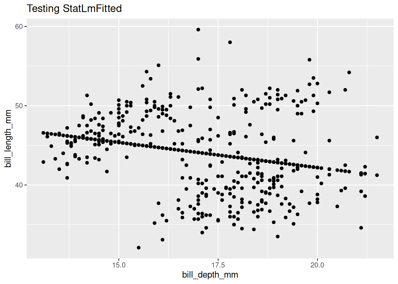
You can test out your Stat using them in ggplot2 geom_*() functions.

penguins |> 
  ggplot() + 
  aes(x = bill_depth_mm,
      y = bill_length_mm) + 
  geom_point() + 
  geom_point(stat = StatLmFitted) + 
  labs(title = "Testing StatLmFitted")

You may have noticed …

that we don’t use “fitted” as the stat argument, which would be more consistent with base ggplot2 documentation. However, if you prefer, you can refer to your newly created Stat this way when testing, i.e. geom_point(stat = "fitted", size = 7).

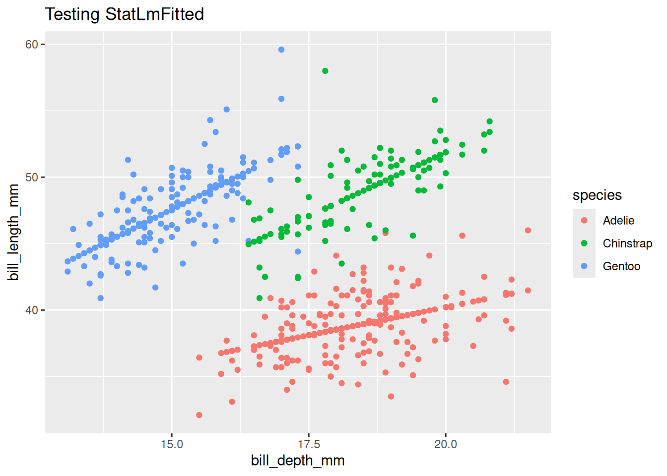
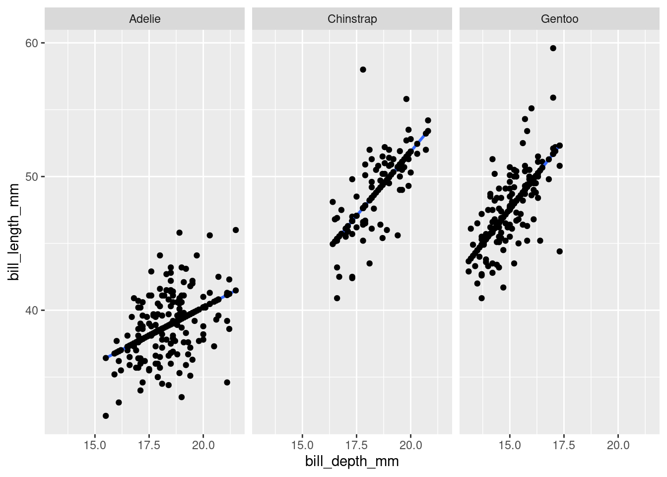
Test group-wise behavior

last_plot() + 
  aes(color = species)

Pro tip: Think about an early exit …

You might be thinking, what we’ve done would already be pretty useful to me. Can I just use my Stat as-is within geom_*() functions?

The short answer is ‘yes’! If you just want to use the Stat yourself locally in a script, there might not be much reason to go on to Step 3, user-facing functions. But if you have a wider audience in mind, i.e. internal to organization or open sourcing in a package, probably a more succinct expression of what functionality you deliver will be useful - i.e. write the user-facing functions.

Pro tip: consider using layer() function to test instead of geom_*(stat = StatNew)

Instead of using a geom_*() function, you might prefer to use the layer() function in your testing step. Occasionally, it’s necessary to go this route; for example, geom_vline() contain no stat argument, but you can use the GeomVline in layer(). If you are teaching this content, using layer() may help you better connect this step with the next, defining the user-facing functions.

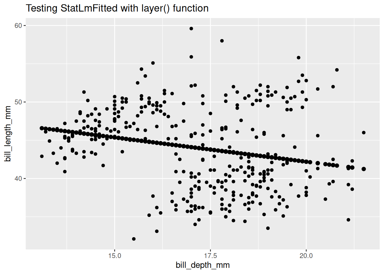
A test of StatFitted using this method follows. You can see it is a little more verbose, as there is no default for the position argument, and setting the size must be handled with a little more care.

penguins |> 
  ggplot() + 
  aes(x = bill_depth_mm,
      y = bill_length_mm) + 
  geom_point() + 
  layer(geom = GeomPoint, 
        stat = StatLmFitted, 
        position = "identity", 
        params = list(size = 2)) + 
  labs(title = "Testing StatLmFitted with layer() function")

Step 3: Define user-facing functions. Test.

In this next section, we define user-facing functions. Doing so is a bit of a mouthful, but see the ‘Pro tip: Use stat_identity definition as a template in this step …’ that follows.

stat_lm_fitted <- function(mapping = NULL, data = NULL, geom = "point", position = "identity", 
    ..., show.legend = NA, inherit.aes = TRUE) {
    layer(data = data, mapping = mapping, stat = StatLmFitted, 
        geom = geom, position = position, show.legend = show.legend, 
        inherit.aes = inherit.aes, params = list(na.rm = FALSE, 
            ...))
}

You may have noticed…

… that the stat_*() function name derives from the Stat objects’s name, but is snake case. So if I wanted a StatBigCircle based stat_*() function, I’d create stat_big_circle().
… that StatIndex is used to define the new layer function, so the computation that defines it, which is to summarize to medians, will be in play before the layer is rendered.
… that "label" is specified as the default for the geom argument in the function. This means that the ggplot2::GeomLabel will be used in the layer unless otherwise specified by the user.

Pro tip. Use stat_identity definition as a template in this step …

…

You may be thinking, defining a new stat_*() function is a mouthful that’s probably hard to reproduce from memory. So you might use stat_identity()’s definition as scaffolding to write your own layer. i.e:

Type stat_identity in your console to print function contents; copy-paste the function definition.
Switch out StatIdentity with your Stat, e.g. StatLmFitted.
Switch out "point" other geom (‘rect’, ‘text’, ‘line’ etc) if needed
Final touch, list2 will error without export from rlang, so update to rlang::list2.

stat_identity

function (mapping = NULL, data = NULL, geom = "point", position = "identity", 
    ..., show.legend = NA, inherit.aes = TRUE) 
{
    layer(data = data, mapping = mapping, stat = StatIdentity, 
        geom = geom, position = position, show.legend = show.legend, 
        inherit.aes = inherit.aes, params = list2(na.rm = FALSE, 
            ...))
}
<bytecode: 0x55a2c9bcc838>
<environment: namespace:ggplot2>

Define geom_*() function

Because users are more accustom to using layers that have the ‘geom’ prefix, you might also define geom with identical properties via aliasing.

geom_lm_fitted <- stat_lm_fitted

Be aware …

… verbatim aliasing as shown above is a bit of a shortcut and assumes that users will use the ‘geom_*()’ function with the stat-geom combination as-is. (For a discussion, see Constructors in ‘Extending ggplot2: A case Study’ in ggplot2: Elegant Graphics for Data Analysis. This section notes, ‘Most ggplot2 users are accustomed to adding geoms, not stats, when building up a plot.’)

An approach that is more consistent with existing guidance would be to hardcode the Geom and allow the user to change the Stat as follows.

# user-facing function
geom_lm_fitted <- function(mapping = NULL, data = NULL, 
                         stat = "lm_fitted", position = "identity", 
                         ..., show.legend = NA, inherit.aes = TRUE) 
{
    layer(data = data, mapping = mapping, stat = stat, 
        geom = GeomPoint, position = position, show.legend = show.legend, 
        inherit.aes = inherit.aes, params = rlang::list2(na.rm = FALSE, 
            ...))
}

However, because it is unexpected to use geom_lm_fitted() with a Stat other than StatLmFitted (doing so would remove the fitted-ness) we think that the verbatim aliasing is a reasonable, time and code saving getting-started approach.

Test/Enjoy functions

penguins %>% 
  ggplot() + 
  aes(x = bill_depth_mm, y = bill_length_mm) +
  geom_point() + 
  geom_smooth(method = "lm") +
  geom_lm_fitted()

`geom_smooth()` using formula = 'y ~ x'

And check out conditionality

penguins %>% 
  ggplot() + 
  aes(x = bill_depth_mm, y = bill_length_mm) +
  geom_point() + 
  geom_smooth(method= "lm", se= F) +
  geom_lm_fitted() + 
  facet_wrap(facets = vars(species))

`geom_smooth()` using formula = 'y ~ x'

Done! Time for a review.

Here is a quick review of the functions and ggproto objects we’ve covered, dropping tests and discussion.

Review

library(tidyverse)

# Step 1. Define compute
compute_group_lm_fitted <- function(data, scales){
  model <- lm(formula = y ~ x, data = data)
  data %>% 
    mutate(y = model$fitted.values)
}


# Step 2. Define Stat
StatLmFitted = ggproto(`_class` = "StatLmFitted",
                      `_inherit` = Stat,
                      required_aes = c("x", "y"),
                      compute_group = compute_group_lm_fitted)

# Step 3. Define user-facing functions

## define stat_*()
stat_lm_fitted <- function(mapping = NULL, data = NULL, 
                         geom = "point", position = "identity", 
                         ..., show.legend = NA, inherit.aes = TRUE) 
{
    layer(data = data, mapping = mapping, stat = StatLmFitted, 
        geom = geom, position = position, show.legend = show.legend, 
        inherit.aes = inherit.aes, params = rlang::list2(na.rm = FALSE, 
            ...))
}

## define geom_*()
geom_lm_fitted <- stat_lm_fitted

Your Turn: Write `geom_residuals()`

Using the geom_lm_fitted Recipe #3 as a reference, try to create a stat_lm_residuals() and convenience geom_fitted() that draws a segment between observed and fitted values for a linear model.

Hint: consider what aesthetics are required for segments. We’ll give you Step 0 this time…

Step 0: use base ggplot2 to get the job done

Step 1: Write compute function. Test.

Step 2: Write Stat.

Step 3: Write user-facing functions.

Congratulations!

If you’ve finished all three recipes, you feel for how Stats can help you build layer functions like stat_residuals and geom_residuals.

The Goal

Example recipe #3: geom_fitted()

Step 0: use base ggplot2 to get the job done

Step 1: Define compute. Test.

Test compute.

Step 2: Define new Stat. Test.

Define Stat.

Test Stat.

Test group-wise behavior

Step 3: Define user-facing functions. Test.

Define geom_*() function

Test/Enjoy functions

And check out conditionality

Done! Time for a review.

Your Turn: Write geom_residuals()

Hint: consider what aesthetics are required for segments. We’ll give you Step 0 this time…

Step 0: use base ggplot2 to get the job done

Step 1: Write compute function. Test.

Step 2: Write Stat.

Step 3: Write user-facing functions.

Congratulations!

Example recipe #3: `geom_fitted()`

Your Turn: Write `geom_residuals()`