Easy geom recipes: a new entry point to ggplot2 extension for statistical educators and their students
Abstract
This project introduces a new introductory material for ggplot2 extension. The tutorial explores six geom_*() extensions in a step-by-step fashion. Three of the extensions are fully worked examples. After each of the worked examples, the tutorial prompts the learner to work through a similar extension.
The tutorial was evaluated by statistics and data analytics educators with substantial R and ggplot2 experience, but without much extension experience.
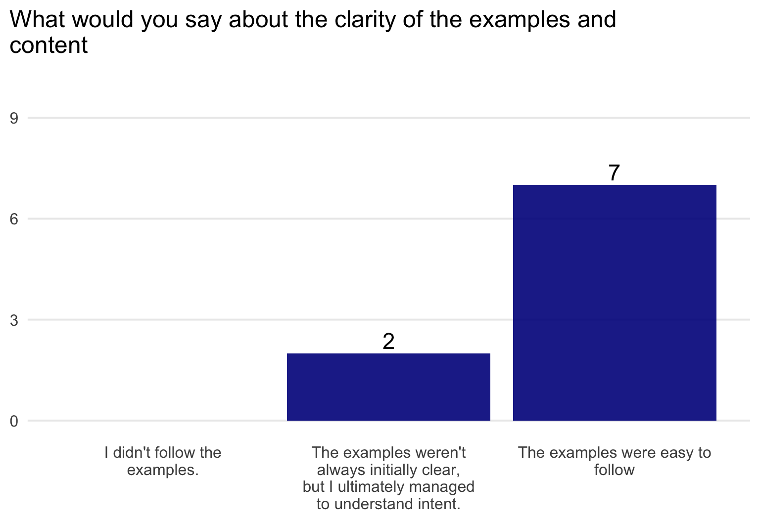
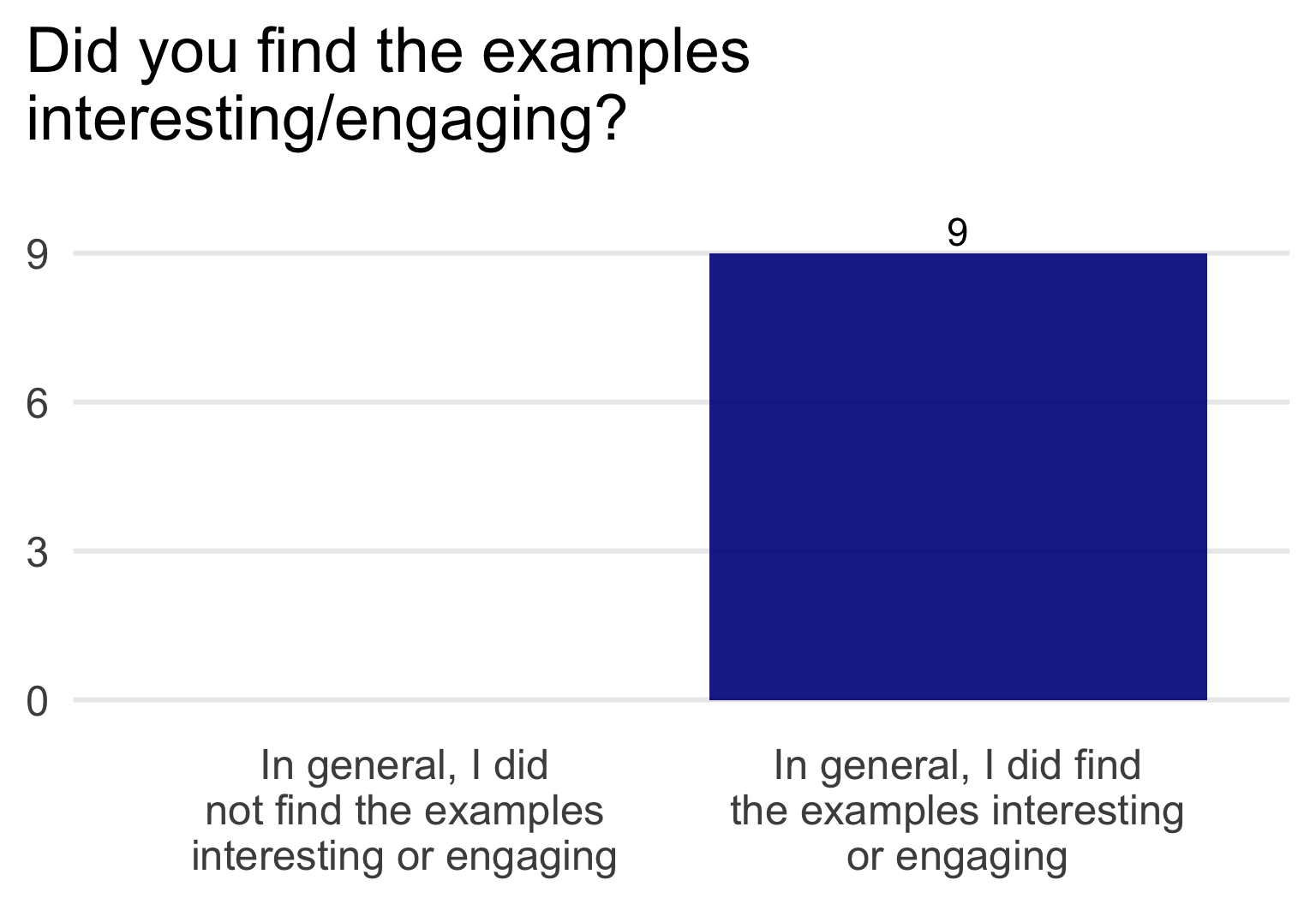
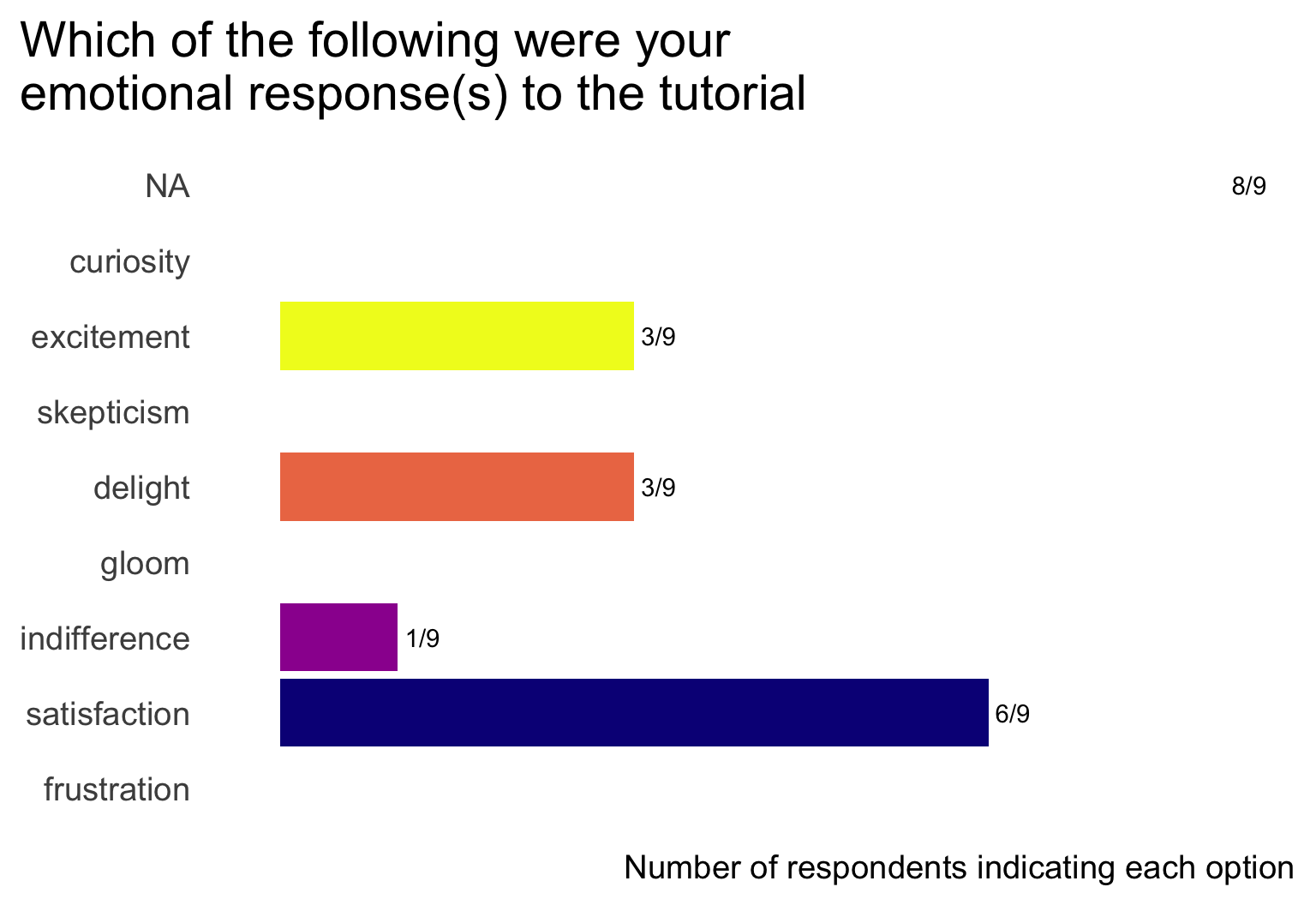
In general, the tutorial was found to be engaging and appropriate in length. The level was judged to be accessible, such that instructors would feel comfortable sharing with advanced students.
Narrative
Using ggplot2 has been described as writing ‘graphical poems’ (Wickham 2010). But we may feel at a loss for ‘words’ when functions we’d like to have don’t exist. The ggplot2 extension system allows us to build new ‘vocabulary’ for fluent expression.
An exciting extension mechanism is that of inheriting from existing, more primitive geoms after performing some calculation.
To get feet wet in this world and provide a taste of patterns for geom*() extension, ‘Easy geom recipes’ provide three basic examples of the geoms that inherit from existing geoms (point, text, segment, etc) along with a practice exercise: https://evamaerey.github.io/easy-geom-recipes/easy_geom_recipes_compute_group.html. With such geoms, calculation is done under the hood by the ggplot2 system. We’ll see how to define a ggproto object.
With new geoms, you can write new graphical poems with exciting new graphical ‘words’!
The tutorial is intended for individuals who already have a working knowledge of the grammar of ggplot2, but may like to build a richer vocabulary for themselves.
Motivation
- ggplot2 extension underutilized.
- inaccessibility to demographic that might really benefit.
- statistical storytelling benefits from greater fluidity that new geoms afford.
- traditional entry point (theme extension) might not be compelling to an audience that might be really productive in extension!
- repetition and numerous examples useful in pedagogical materials
Tutorial form
The introductory tutorial took the form of three examples where a geom_*() is successfully created in a step-by-step fashion. After each example, the learner is prompted to create an additional geom that is computationally similar to the example.
Our recipes take the form:
- Step 0. Get the job done with ‘base’ ggplot2. It’s a good idea to clarify what needs to happen without getting into the extension architecture
- Step 1. Write a computation function. Wrap the necessary computation into a function that your target geom_*() function will perform. We focus on ‘compute_group’ computation only in this tutorial.
- Step 2. Define a ggproto object. ggproto objects allow your extension to work together with base ggplot2 functions! You’ll use the computation function from step 1 to help define it.
- Step 3. Write your geom function! You’re ready to write your function. You will incorporate the ggproto from step 2 and also define which more primitive geom (point, text, segment etc) you want other behaviors to inherit from.
- Step 4. Test/Enjoy! Take your new geom for a spin! Check out group-wise computation behavior!
Evaluation
To test the tutorial, we approached statistics and data analytics educators that we believed would have substantial experience with R and ggplot2 but not necessarily with ggplot2 extension. The study includes nine participants that completed the study and responded to a survey about the tutorial. Eight of the participants were also able to participate in focus group discussions following their completion of the the tutorial and survey.
Participant profiles
Recruited participants generally had substantial experience teaching data analytics.
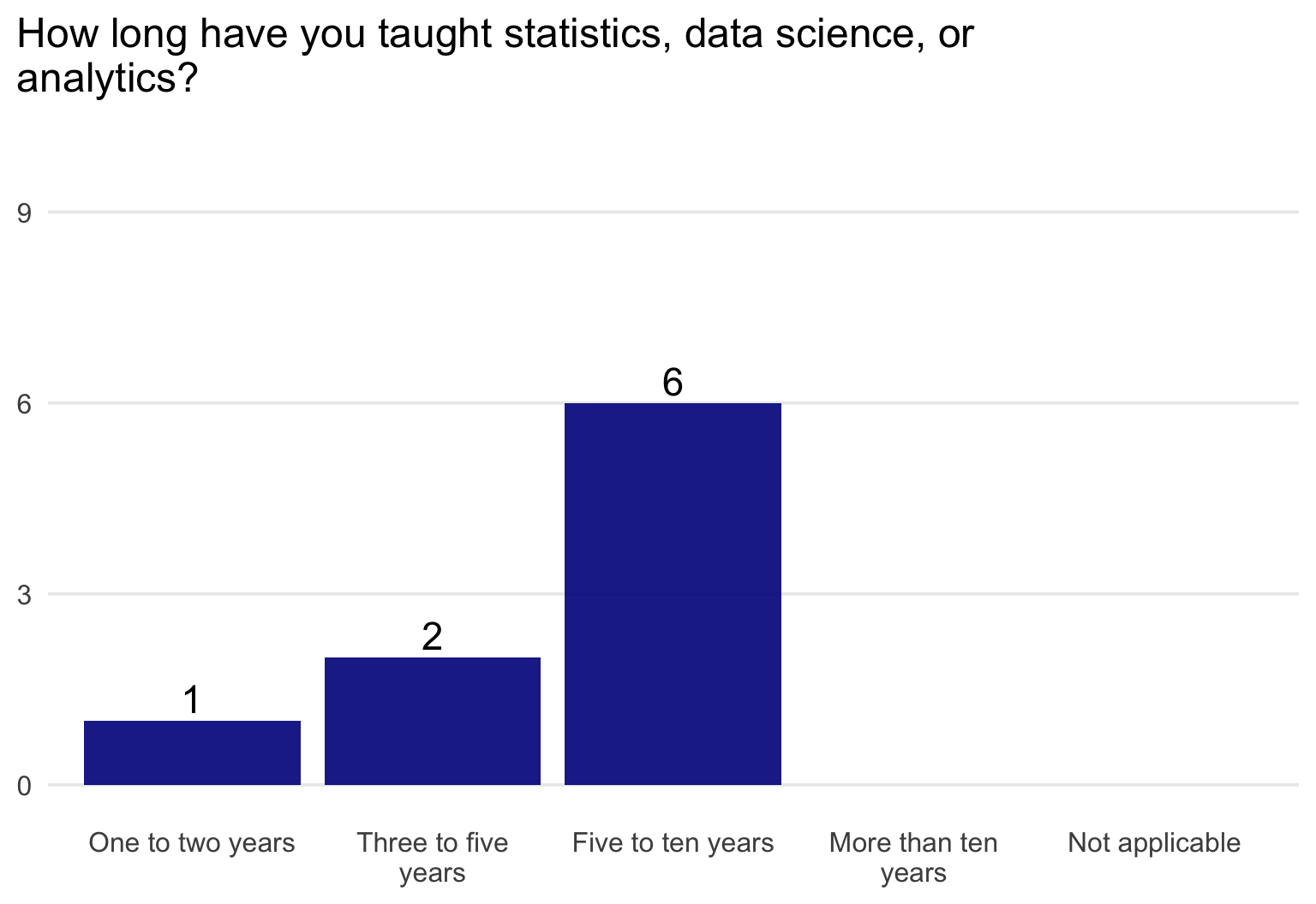
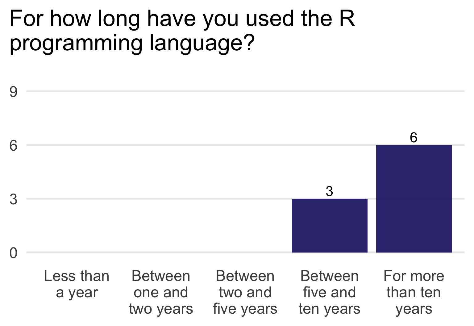
Study participants all had substantial experience. All had at least five years programming in the R statistical language, with the majority having more than ten years of experience.
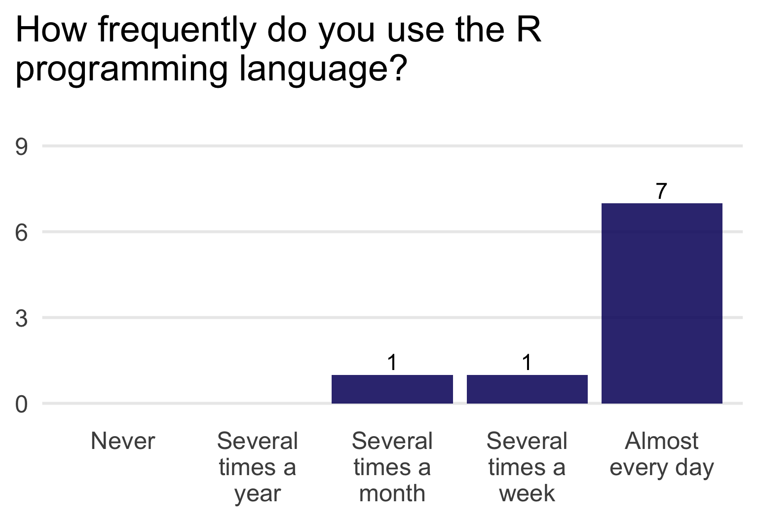
All but one of the participants use the R language several times a week, with many using the language ‘almost every day’.
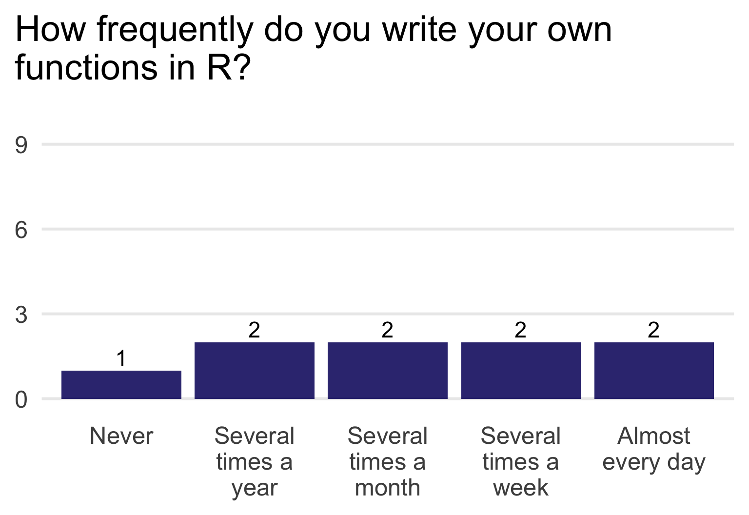
With respect to writing functions, most of the group had experience writing functions, though the frequency was not as great as with using R and ggplot2.
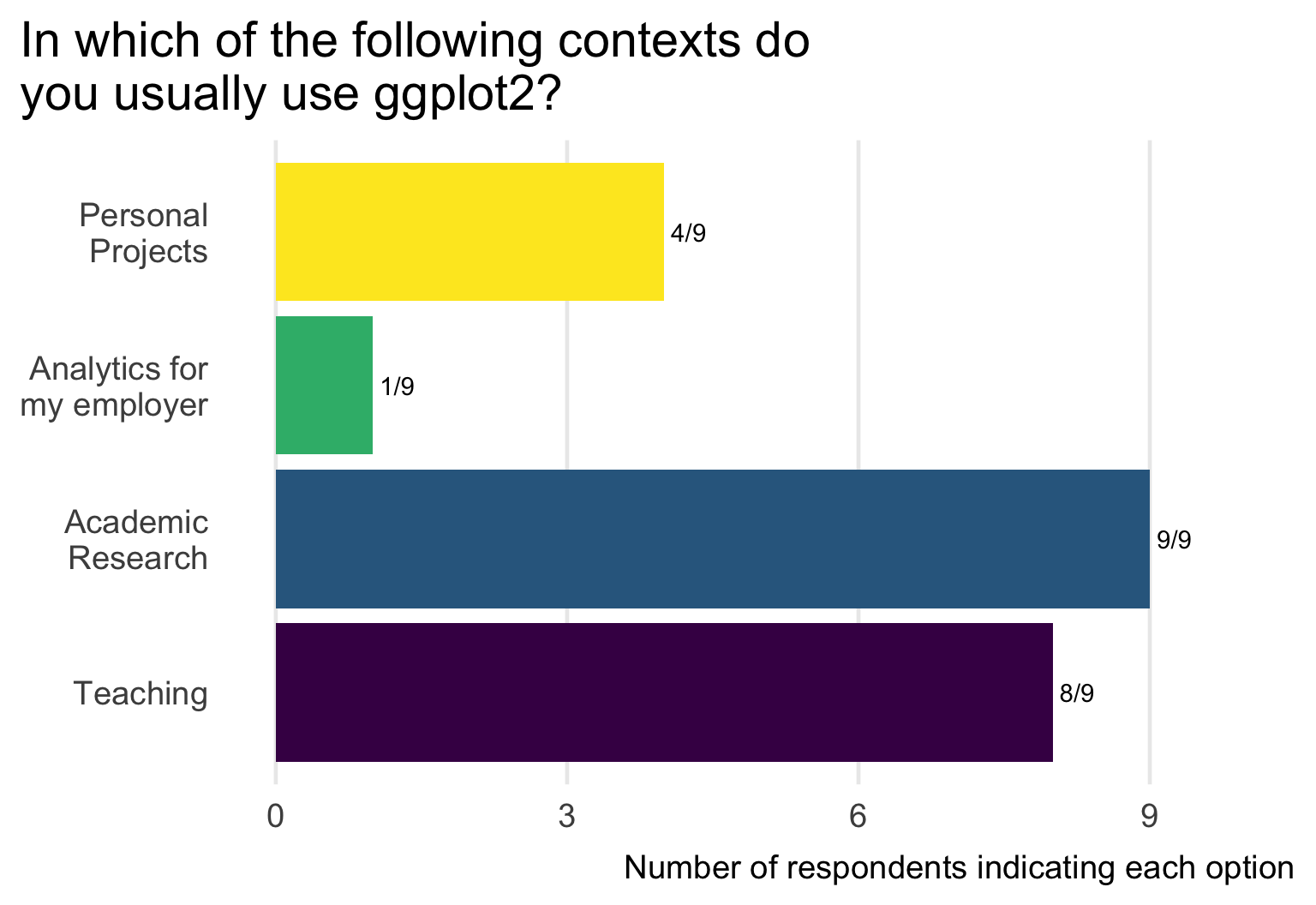
The respondents use ggplot2 in a variety of contexts; notably they all use it in academic research and eight of nine used it in teaching.
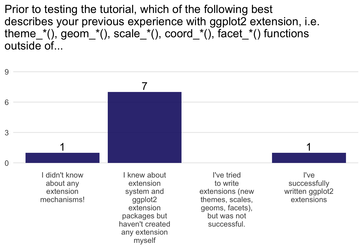
However, participants in general had little or no with writing ggplot2 extensions. Seven of the nine participants were aware of extension packages but had not attempted to write their own extension. One participant had written ggplot2 extensions prior to the tutorial.
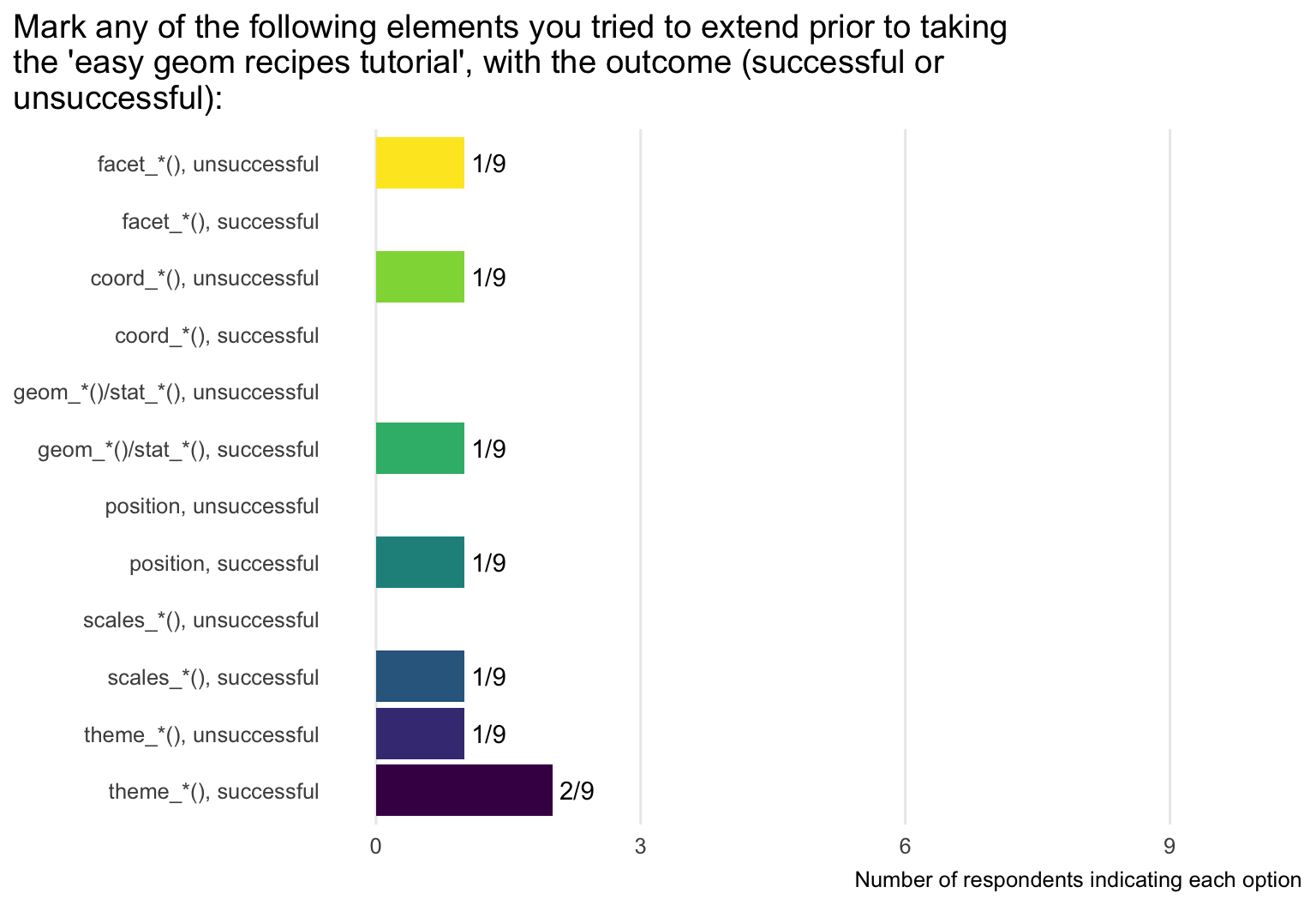
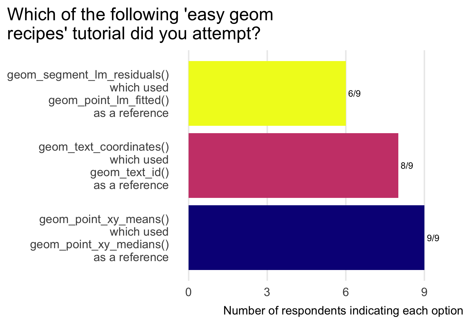
The following figure shows attempts and successes or failures in the different ggplot2 extension areas.
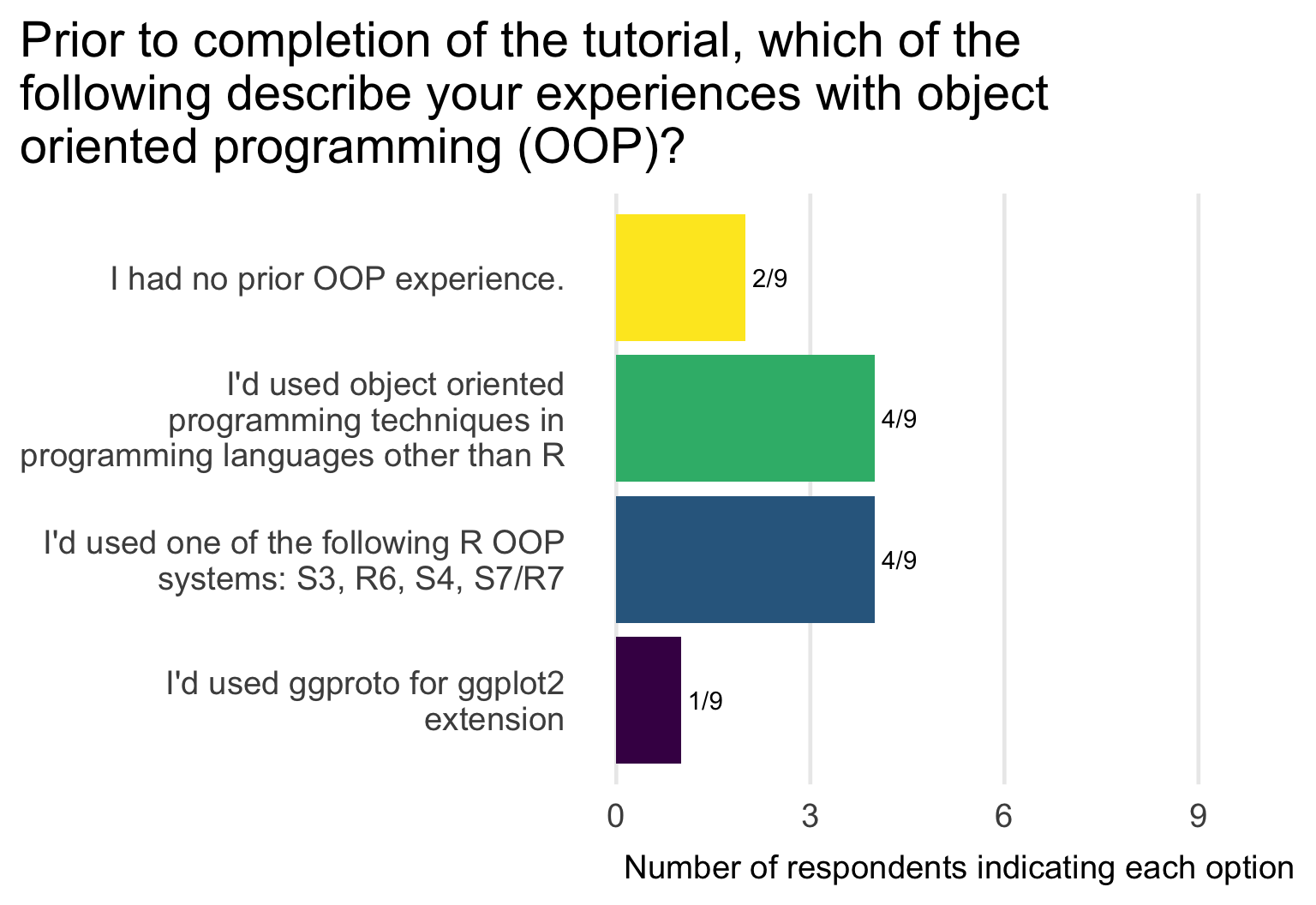
The participants had a variety of experiences with object oriented programming. About half had experience with OOP in R in general, but only one had used the ggproto OOP system.
Tutorial assessment
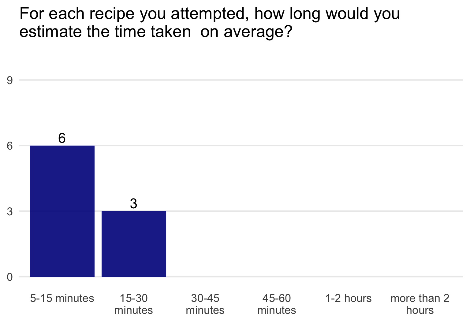
Most participants indicated the tutorial taking them a short amount of time. Six of nine said that on average, each of the recipes took less than 15 minutes to complete. The remaining three participants responded that the recipes took between 15 and 30 minutes on average.
The first prompt geom_point_xy_means exercise was completed by all participants; and all but one completed the geom_text_coordinates() exercise. Several participants failed complete the last recipe (residuals).
Appendix, example exercise
For clarity, I include one of the three exercises in the ‘easy geom recipes’ extension tutorial. First an ‘example recipe’ geom_label_id() is provided, with the step 0-4 guideposts. Then, the student is prompted to create geom_text_coordinates().
Thanks to Claus Wilke, June Choe, Teun van der Brand, Isabella Velasquez, Cosima Meyer, Eric Reder, Dusty Turner, and Rebecca Conley for review, pre-testing, and useful feedback on earlier versions of the tutorial.
# Example recipe #2:  `geom_label_id()`

---

## Step 0: use base ggplot2 to get the job done

```{r}
#| label: cars
# step 0.a
cars %>%
  mutate(id_number = 1:n()) %>%
  ggplot() +
  aes(x = speed, y = dist) +
  geom_point() +
  geom_label(aes(label = id_number),
             hjust = 1.2)

# step 0.b
layer_data(last_plot(), i = 2) %>%
  head()
```


---

## Step 1: computation

```{r}
#| label: compute_group_row_number
# you won't use the scales argument, but ggplot will later
compute_group_row_number <- function(data, scales){

  data %>%
    # add an additional column called label
    # the geom we inherit from requires the label aesthetic
    mutate(label = 1:n())

}

# step 1b test the computation function
cars %>%
  # input must have required aesthetic inputs as columns
  rename(x = speed, y = dist) %>%
  compute_group_row_number() %>%
  head()
```

---

## Step 2: define ggproto

```{r}
#| label: StatRownumber
StatRownumber <- ggplot2::ggproto(`_class` = "StatRownumber",
                                  `_inherit` = ggplot2::Stat,
                                  required_aes = c("x", "y"),
                                  compute_group = compute_group_row_number)
```


---

## Step 3: define geom_* function


- define the stat and geom for your layer

```{r}
#| label: geom_label_row_number
geom_label_row_number <- function(mapping = NULL, data = NULL,
                           position = "identity", na.rm = FALSE,
                           show.legend = NA,
                           inherit.aes = TRUE, ...) {
  ggplot2::layer(
    stat = StatRownumber, # proto object from Step 2
    geom = ggplot2::GeomLabel, # inherit other behavior, this time Label
    data = data,
    mapping = mapping,
    position = position,
    show.legend = show.legend,
    inherit.aes = inherit.aes,
    params = list(na.rm = na.rm, ...)
  )
}
```


---

## Step 4: Enjoy! Use your function

```{r}
#| label: enjoy_again
cars %>%
  ggplot() +
  aes(x = speed, y = dist) +
  geom_point() +
  geom_label_row_number(hjust = 1.2) # function in action
```

### And check out conditionality!

```{r}
#| label: conditional_compute
last_plot() +
  aes(color = dist > 60) # Computation is within group
```


---

# Task #2: create `geom_text_coordinates()`

Using recipe #2 as a reference, can you create the function `geom_text_coordinates()`.

--

- geom should label point with its coordinates '(x, y)'
- geom should have behavior of geom_text (not geom_label)


Hint:

```{r}
paste0("(", 1, ", ",3., ")")
```

```{r}
# step 0: use base ggplot2

# step 1: write your compute_group function (and test)

# step 2: write ggproto with compute_group as an input

# step 3: write your geom_*() function with ggproto as an input

# step 4: enjoy!

```