ggalluvial

ggplot2 allows you build up your plot bit by bit – to write ‘graphical poems’ (Wickham 2010). It is easy to gain insights simply by 1. defining a data set to look at, 2. the aesthetics (x position, y position, color, size, etc) that should represent variables from that data, and 3. what geometric marks should take on those aesthetics. Inspired by this incrementalism, frameworks like camcorder, flipbookr, codehover exist to capture plot composition.

library(ggalluvial)
library(ggplot2)
titanic_wide <- data.frame(Titanic)
head(titanic_wide)

  Class    Sex   Age Survived Freq
1   1st   Male Child       No    0
2   2nd   Male Child       No    0
3   3rd   Male Child       No   35
4  Crew   Male Child       No    0
5   1st Female Child       No    0
6   2nd Female Child       No    0

#>   Class    Sex   Age Survived Freq
#> 1   1st   Male Child       No    0
#> 2   2nd   Male Child       No    0
#> 3   3rd   Male Child       No   35
#> 4  Crew   Male Child       No    0
#> 5   1st Female Child       No    0
#> 6   2nd Female Child       No    0
#> 

StatStratum$default_aes <- aes(label = after_stat(stratum))
geom_stratum_text <- function(...){geom_text(stat = StatStratum, ...)}

library(ggplot2)
library(ggalluvial)

GeomStratum$default_aes # hardcoded

Aesthetic mapping: 
* `size`      -> 0.5
* `linewidth` -> 0.5
* `linetype`  -> 1
* `colour`    -> "black"
* `fill`      -> "white"
* `alpha`     -> 1

GeomRect$default_aes

Aesthetic mapping: 
* `colour`    -> NA
* `fill`      -> `from_theme(col_mix(ink, paper, 0.35))`
* `linewidth` -> `from_theme(borderwidth)`
* `linetype`  -> `from_theme(bordertype)`
* `alpha`     -> NA

GeomStratum$default_aes <- GeomRect$default_aes
GeomStratum$default_aes <- modifyList(GeomRect$default_aes, 
                                      aes(color = from_theme(ggplot2:::col_mix(ink, paper, 0.15))))

Here is a graphical poem!

ggplot(data = titanic_wide) + # Ok Lets look at this titanic data
  aes(y = Freq, axis1 = Sex, axis2 = Survived) + # Here some variables of interest
  ggchalkboard:::theme_slateboard(base_size = 18) + # in a alluvial plot first look
  geom_alluvium() + # And we are ready to look at flow
  geom_stratum(aes(fill = NULL)) + # And we can label our stratum axes
  geom_stratum_text() + # Add stratum labels
  aes(axis1 = Age) + # look at age to survival
  aes(axis1 = Class) + # look at class to survival
  aes(axis1 = Age, axis2 = Class, axis3 = Survived) + # age to class to survival
  aes(axis1 = Sex, axis2 = Age, axis3 = Class, axis4 = Survived) + # a train
  aes(fill = Sex) + # Track sex throughout
  guides(fill = "none") + # remove fill guide as axis1 is labeled
  scale_x_discrete(limits = c("Sex", "Age", "Class", "Survived"), expand = c(.1, .1)) + # adjusting the x axis
  labs(x = "Demographic") + # An overall label for x axis
  labs(caption = "Passengers on the maiden voyage of the Titanic") + # adding a caption 
  aes(axis1 = fct_rev(Sex)) + # minimize flow crossing
  aes(axis4 = fct_rev(Survived)) + # minimize flow crossing
  aes(axis2 = NULL) + # remove Age
  aes(axis1 = ifelse(Sex == "Female" | Age == "Child", "Female or Child", "Male Adult")) + # Replace axis 1
    scale_x_discrete(limits = c("Sex & Age", "Class", "Survived"), expand = c(.2, .1)) + # adjusting the x axis
  aes(fill = ifelse(Sex == "Female" | Age == "Child", "Female or Child", "Male Adult")) # More 

Closeread helps walk people through and digest ideas suggesting a synergy with the gg world. With Closereads, maybe we can read this graphical poem ‘aloud’, and reflect on it a bit in plain language as we go. Here is a generic way to write out what closereads requires for creating plot output and referring to it.

cr_last_plot_construction <- ':::{focus-on="cr-.PLOTXXX"}\n.COMMENT, using `.CODE`\n:::\n\n:::{#cr-.PLOTXXX}\n```{r .PLOTXXX}\n.LEADING\n  .CODE\n```\n:::\n'  

cr_last_plot_construction |> cat()

:::{focus-on="cr-.PLOTXXX"}
.COMMENT, using `.CODE`
:::

:::{#cr-.PLOTXXX}
```{r .PLOTXXX}
.LEADING
  .CODE
```
:::

Then we can look at our complete ‘graphical poem’, parse it, choreograph a line by line reveal - thanks Garrick and Emi for showing the way using powerful knitr::knit_code$get in Xaringan context! https://emitanaka.rbind.io/post/knitr-knitr-code/ At this point we aren’t being really careful with code parsing or replacement; flipbookr internals has some nicer parsing that might be useable and allow more incremental reveals in other contexts like datamanipulation and table creation. In contrast to the full reiterated code that we show in flipbookr w/ Xaringan w/ plot, we’ll use last_plot() + new_code() below. It just feels like a better fit.

knitr::knit_code$get("walkthrough") |>
  tibble(code_raw = _) |>
  mutate(comment = str_extract(code_raw, "#.+$")) |>
  mutate(comment = str_remove(comment, "#")) |>
  mutate(code = str_remove(code_raw, "\\+ #.+$|#.+$")) |>
  mutate(index = row_number()) |>
  mutate(plot_name = paste("walkthrough", sep = "-", index)) |>
  mutate(to_cr = cr_last_plot_construction) |>
  mutate(to_cr = str_replace_all(to_cr, ".PLOTXXX", plot_name)) |>
  mutate(to_cr = str_replace(to_cr, ".COMMENT", comment)) |>
  mutate(to_cr = str_replace_all(to_cr, ".CODE", code)) |>
  mutate(to_cr = str_replace(to_cr, ".LEADING", ifelse(index == 1, "", "last_plot() +"))) |>
  pull(to_cr) -> 
to_closeread

to_closeread

 [1] ":::{focus-on=\"cr-walkthrough-1\"}\n Ok Lets look at this titanic data, using `ggplot(data = titanic_wide) `\n:::\n\n:::{#cr-walkthrough-1}\n```{r walkthrough-1}\n\n  ggplot(data = titanic_wide) \n```\n:::\n"                                                                                                                                       
 [2] ":::{focus-on=\"cr-walkthrough-2\"}\n Here some variables of interest, using `  aes(y = Freq, axis1 = Sex, axis2 = Survived) `\n:::\n\n:::{#cr-walkthrough-2}\n```{r walkthrough-2}\nlast_plot() +\n    aes(y = Freq, axis1 = Sex, axis2 = Survived) \n```\n:::\n"                                                                                      
 [3] ":::{focus-on=\"cr-walkthrough-3\"}\n in a alluvial plot first look, using `  ggchalkboard:::theme_slateboard(base_size = 18) `\n:::\n\n:::{#cr-walkthrough-3}\n```{r walkthrough-3}\nlast_plot() +\n    ggchalkboard:::theme_slateboard(base_size = 18) \n```\n:::\n"                                                                                  
 [4] ":::{focus-on=\"cr-walkthrough-4\"}\n And we are ready to look at flow, using `  geom_alluvium() `\n:::\n\n:::{#cr-walkthrough-4}\n```{r walkthrough-4}\nlast_plot() +\n    geom_alluvium() \n```\n:::\n"                                                                                                                                               
 [5] ":::{focus-on=\"cr-walkthrough-5\"}\n And we can label our stratum axes, using `  geom_stratum(aes(fill = NULL)) `\n:::\n\n:::{#cr-walkthrough-5}\n```{r walkthrough-5}\nlast_plot() +\n    geom_stratum(aes(fill = NULL)) \n```\n:::\n"                                                                                                                
 [6] ":::{focus-on=\"cr-walkthrough-6\"}\n Add stratum labels, using `  geom_stratum_text() `\n:::\n\n:::{#cr-walkthrough-6}\n```{r walkthrough-6}\nlast_plot() +\n    geom_stratum_text() \n```\n:::\n"                                                                                                                                                     
 [7] ":::{focus-on=\"cr-walkthrough-7\"}\n look at age to survival, using `  aes(axis1 = Age) `\n:::\n\n:::{#cr-walkthrough-7}\n```{r walkthrough-7}\nlast_plot() +\n    aes(axis1 = Age) \n```\n:::\n"                                                                                                                                                      
 [8] ":::{focus-on=\"cr-walkthrough-8\"}\n look at class to survival, using `  aes(axis1 = Class) `\n:::\n\n:::{#cr-walkthrough-8}\n```{r walkthrough-8}\nlast_plot() +\n    aes(axis1 = Class) \n```\n:::\n"                                                                                                                                                
 [9] ":::{focus-on=\"cr-walkthrough-9\"}\n age to class to survival, using `  aes(axis1 = Age, axis2 = Class, axis3 = Survived) `\n:::\n\n:::{#cr-walkthrough-9}\n```{r walkthrough-9}\nlast_plot() +\n    aes(axis1 = Age, axis2 = Class, axis3 = Survived) \n```\n:::\n"                                                                                   
[10] ":::{focus-on=\"cr-walkthrough-10\"}\n a train, using `  aes(axis1 = Sex, axis2 = Age, axis3 = Class, axis4 = Survived) `\n:::\n\n:::{#cr-walkthrough-10}\n```{r walkthrough-10}\nlast_plot() +\n    aes(axis1 = Sex, axis2 = Age, axis3 = Class, axis4 = Survived) \n```\n:::\n"                                                                       
[11] ":::{focus-on=\"cr-walkthrough-11\"}\n Track sex throughout, using `  aes(fill = Sex) `\n:::\n\n:::{#cr-walkthrough-11}\n```{r walkthrough-11}\nlast_plot() +\n    aes(fill = Sex) \n```\n:::\n"                                                                                                                                                        
[12] ":::{focus-on=\"cr-walkthrough-12\"}\n remove fill guide as axis1 is labeled, using `  guides(fill = \"none\") `\n:::\n\n:::{#cr-walkthrough-12}\n```{r walkthrough-12}\nlast_plot() +\n    guides(fill = \"none\") \n```\n:::\n"                                                                                                                       
[13] ":::{focus-on=\"cr-walkthrough-13\"}\n adjusting the x axis, using `  scale_x_discrete(limits = c(\"Sex\", \"Age\", \"Class\", \"Survived\"), expand = c(.1, .1)) `\n:::\n\n:::{#cr-walkthrough-13}\n```{r walkthrough-13}\nlast_plot() +\n    scale_x_discrete(limits = c(\"Sex\", \"Age\", \"Class\", \"Survived\"), expand = c(.1, .1)) \n```\n:::\n"
[14] ":::{focus-on=\"cr-walkthrough-14\"}\n An overall label for x axis, using `  labs(x = \"Demographic\") `\n:::\n\n:::{#cr-walkthrough-14}\n```{r walkthrough-14}\nlast_plot() +\n    labs(x = \"Demographic\") \n```\n:::\n"                                                                                                                             
[15] ":::{focus-on=\"cr-walkthrough-15\"}\n adding a caption , using `  labs(caption = \"Passengers on the maiden voyage of the Titanic\") `\n:::\n\n:::{#cr-walkthrough-15}\n```{r walkthrough-15}\nlast_plot() +\n    labs(caption = \"Passengers on the maiden voyage of the Titanic\") \n```\n:::\n"                                                     
[16] ":::{focus-on=\"cr-walkthrough-16\"}\n minimize flow crossing, using `  aes(axis1 = fct_rev(Sex)) `\n:::\n\n:::{#cr-walkthrough-16}\n```{r walkthrough-16}\nlast_plot() +\n    aes(axis1 = fct_rev(Sex)) \n```\n:::\n"                                                                                                                                  
[17] ":::{focus-on=\"cr-walkthrough-17\"}\n minimize flow crossing, using `  aes(axis4 = fct_rev(Survived)) `\n:::\n\n:::{#cr-walkthrough-17}\n```{r walkthrough-17}\nlast_plot() +\n    aes(axis4 = fct_rev(Survived)) \n```\n:::\n"                                                                                                                        
[18] ":::{focus-on=\"cr-walkthrough-18\"}\n remove Age, using `  aes(axis2 = NULL) `\n:::\n\n:::{#cr-walkthrough-18}\n```{r walkthrough-18}\nlast_plot() +\n    aes(axis2 = NULL) \n```\n:::\n"                                                                                                                                                              
[19] ":::{focus-on=\"cr-walkthrough-19\"}\n Replace axis 1, using `  aes(axis1 = ifelse(Sex == \"Female\" | Age == \"Child\", \"Female or Child\", \"Male Adult\")) `\n:::\n\n:::{#cr-walkthrough-19}\n```{r walkthrough-19}\nlast_plot() +\n    aes(axis1 = ifelse(Sex == \"Female\" | Age == \"Child\", \"Female or Child\", \"Male Adult\")) \n```\n:::\n"
[20] ":::{focus-on=\"cr-walkthrough-20\"}\n adjusting the x axis, using `    scale_x_discrete(limits = c(\"Sex & Age\", \"Class\", \"Survived\"), expand = c(.2, .1)) `\n:::\n\n:::{#cr-walkthrough-20}\n```{r walkthrough-20}\nlast_plot() +\n      scale_x_discrete(limits = c(\"Sex & Age\", \"Class\", \"Survived\"), expand = c(.2, .1)) \n```\n:::\n"  
[21] ":::{focus-on=\"cr-walkthrough-21\"}\n More , using `  aes(fill = ifelse(Sex == \"Female\" | Age == \"Child\", \"Female or Child\", \"Male Adult\")) `\n:::\n\n:::{#cr-walkthrough-21}\n```{r walkthrough-21}\nlast_plot() +\n    aes(fill = ifelse(Sex == \"Female\" | Age == \"Child\", \"Female or Child\", \"Male Adult\")) \n```\n:::\n"           

Okay, ready for the closeread demonstration! (Comparing flipbookr/xaringan implementation what we are doing here, there’s probably greater focus on narration.) We’ll use knitr::knit() inline to get this done - paste(knitr::knit(text = to_closeread, quiet = F), collapse = "\n\n")

Ok Lets look at this titanic data, using ggplot(data = titanic_wide)

Here some variables of interest, using aes(y = Freq, axis1 = Sex, axis2 = Survived)

in a alluvial plot first look, using ggchalkboard:::theme_slateboard(base_size = 18)

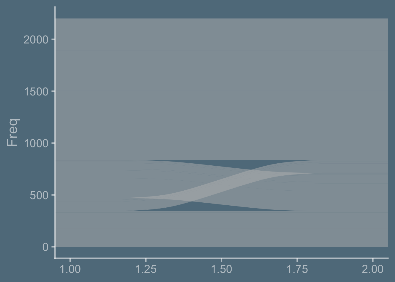
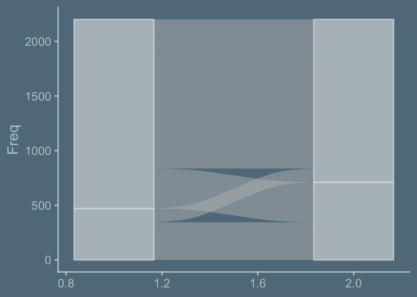
And we are ready to look at flow, using geom_alluvium()

And we can label our stratum axes, using geom_stratum(aes(fill = NULL))

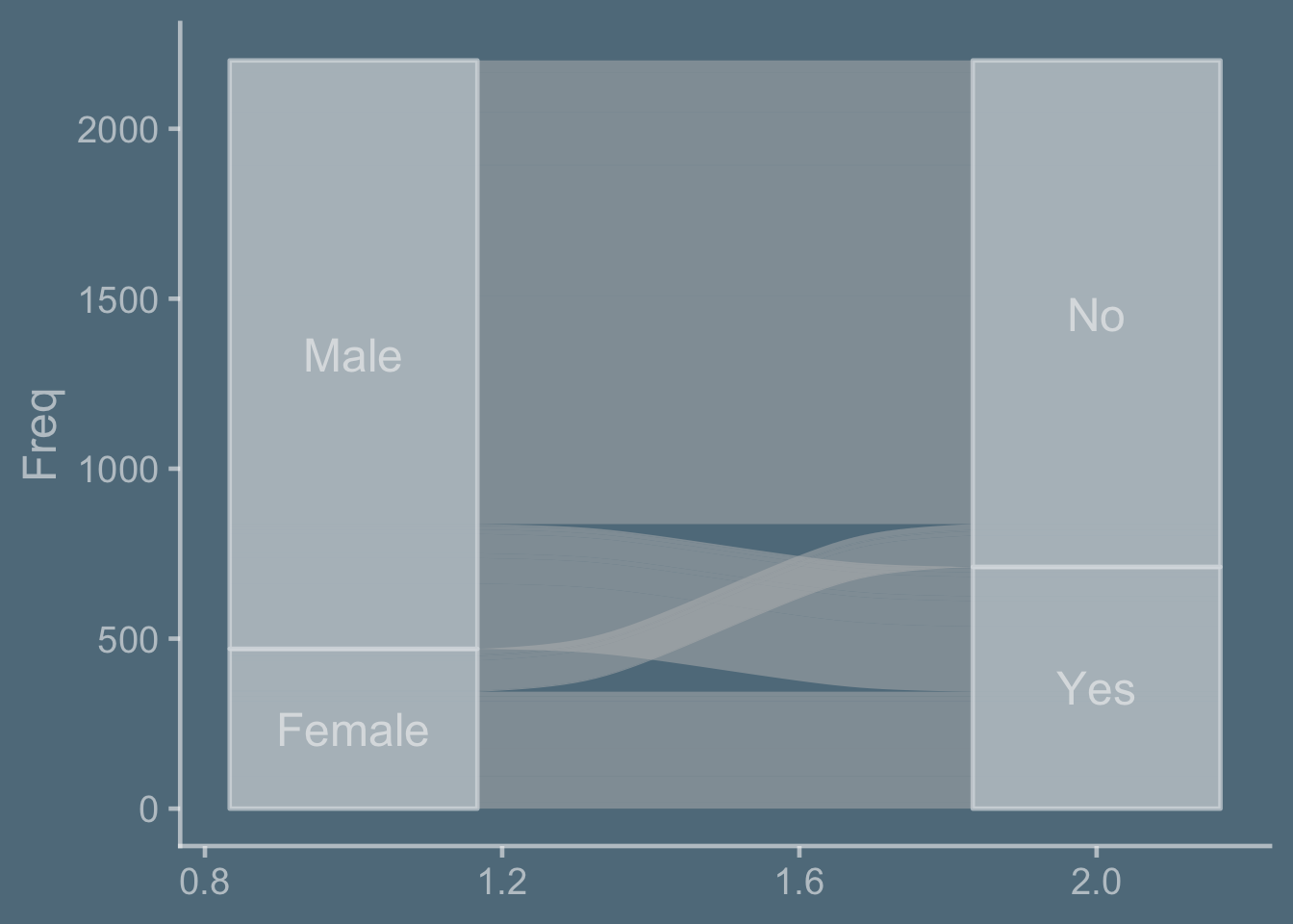
Add stratum labels, using geom_stratum_text()

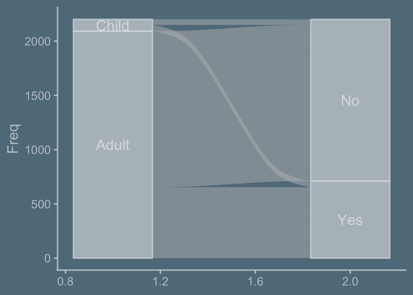
look at age to survival, using aes(axis1 = Age)

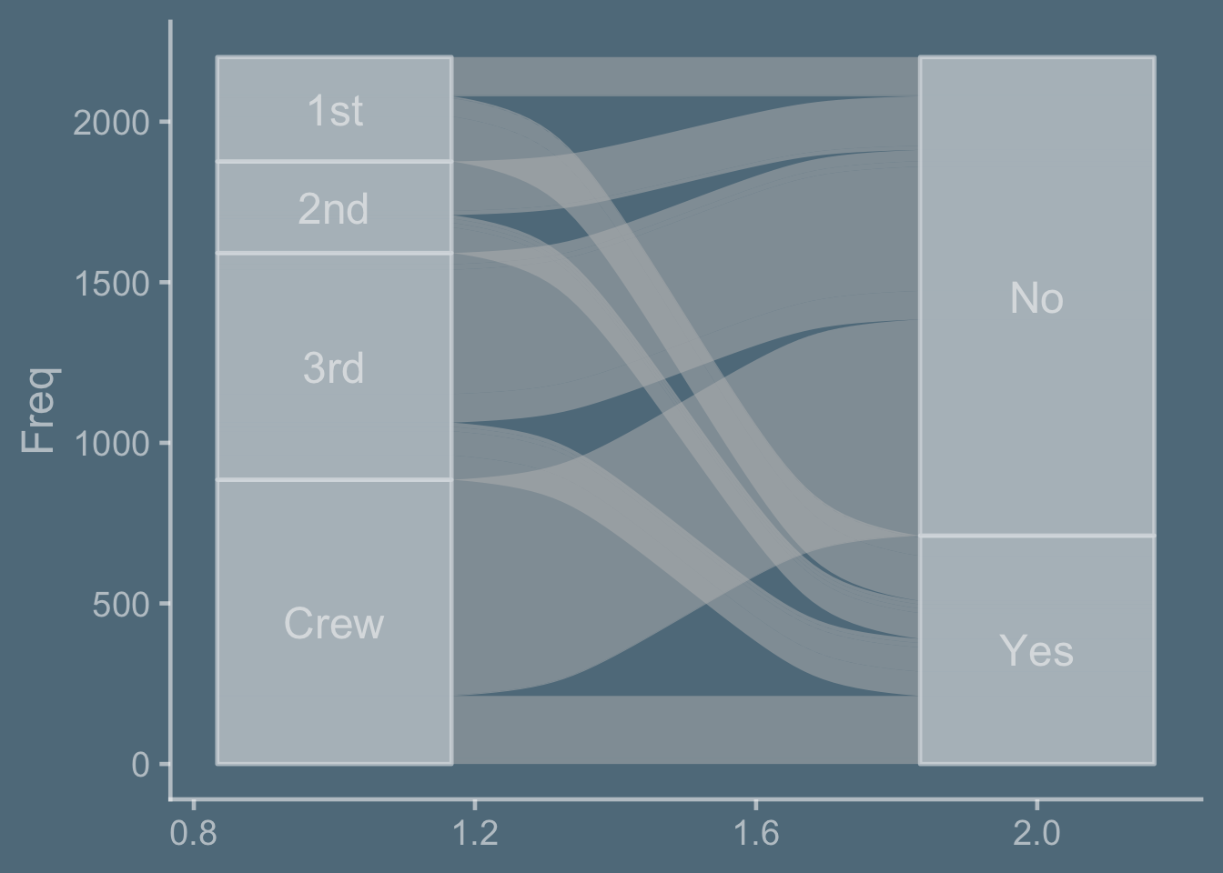
look at class to survival, using aes(axis1 = Class)

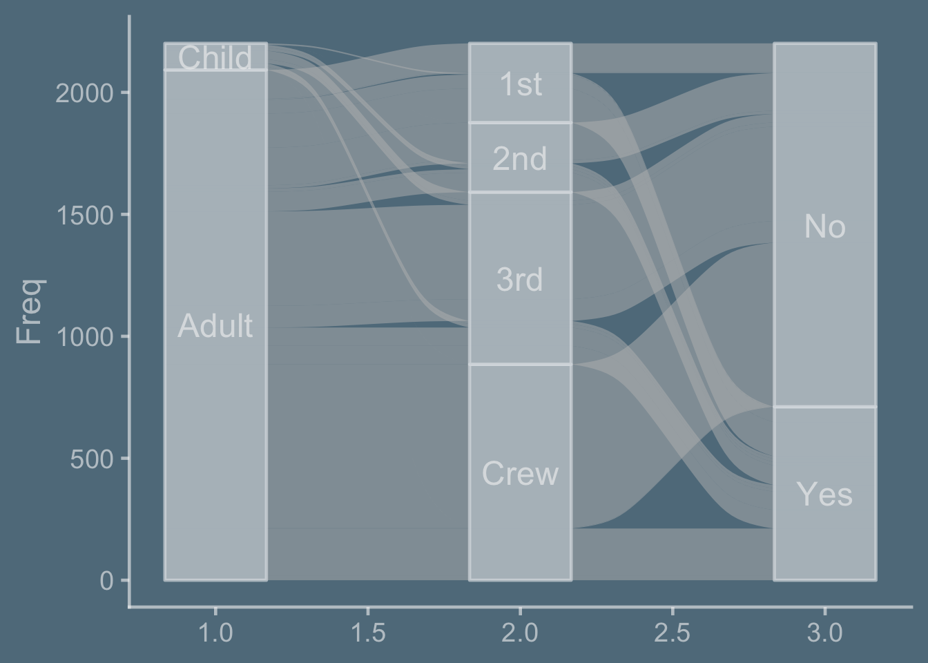
age to class to survival, using aes(axis1 = Age, axis2 = Class, axis3 = Survived)

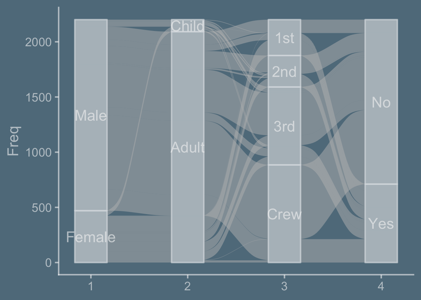
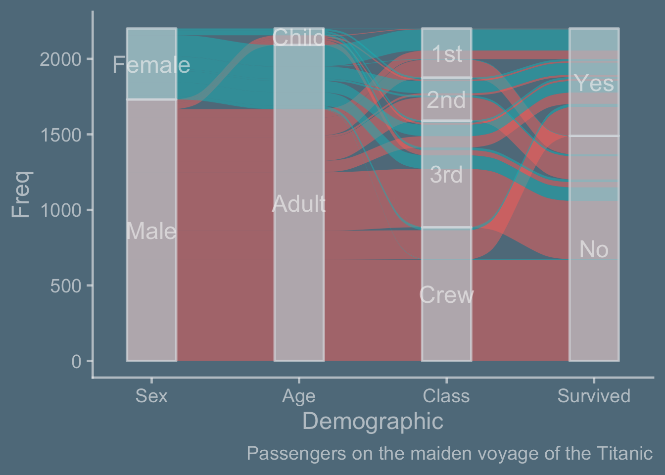
a train, using aes(axis1 = Sex, axis2 = Age, axis3 = Class, axis4 = Survived)

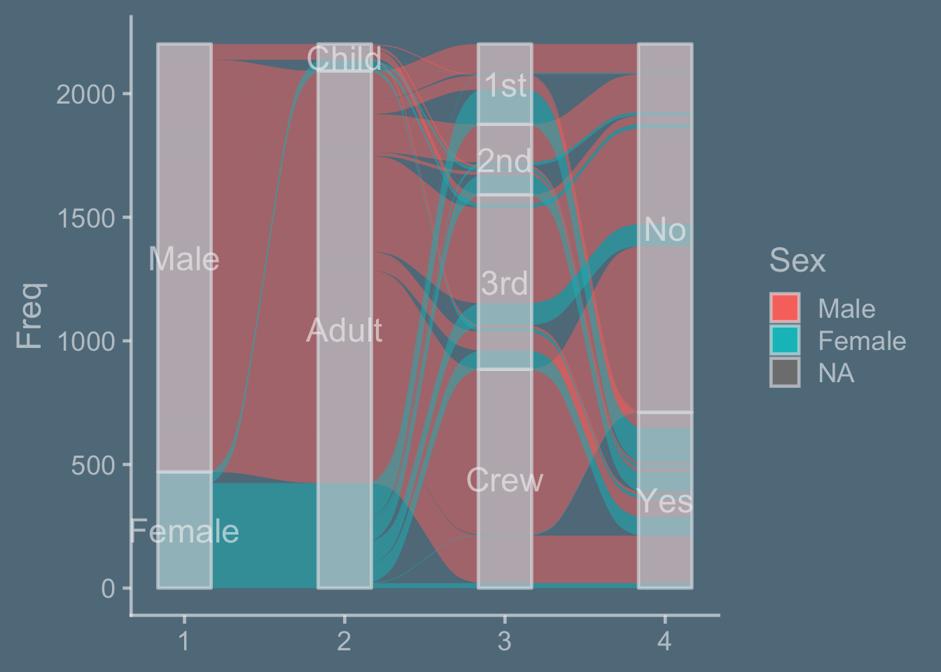
Track sex throughout, using aes(fill = Sex)

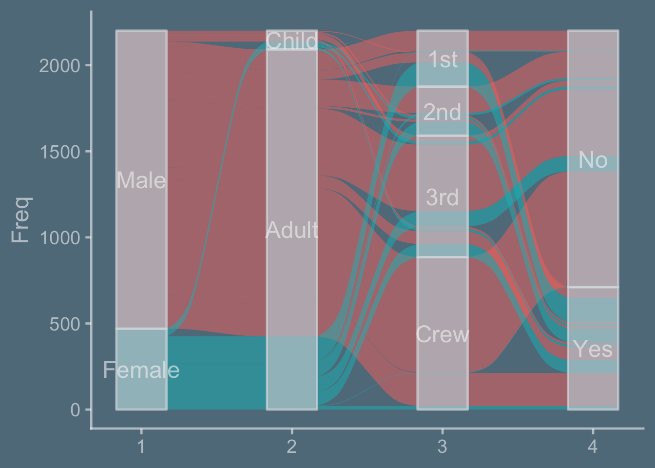
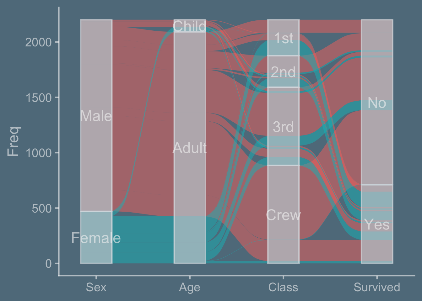
remove fill guide as axis1 is labeled, using guides(fill = "none")

adjusting the x axis, using scale_x_discrete(limits = c("Sex", "Age", "Class", "Survived"), expand = c(.1, .1))

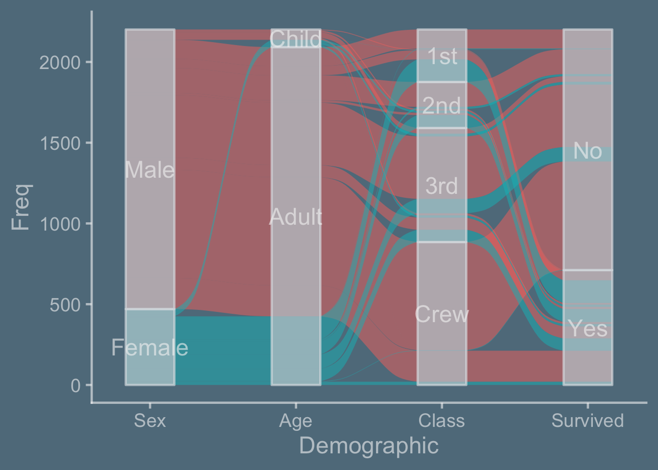
An overall label for x axis, using labs(x = "Demographic")

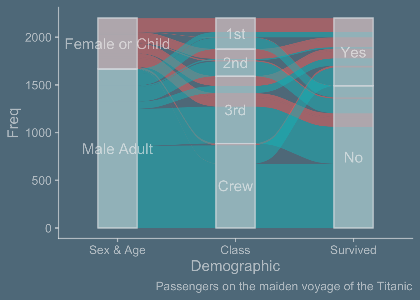
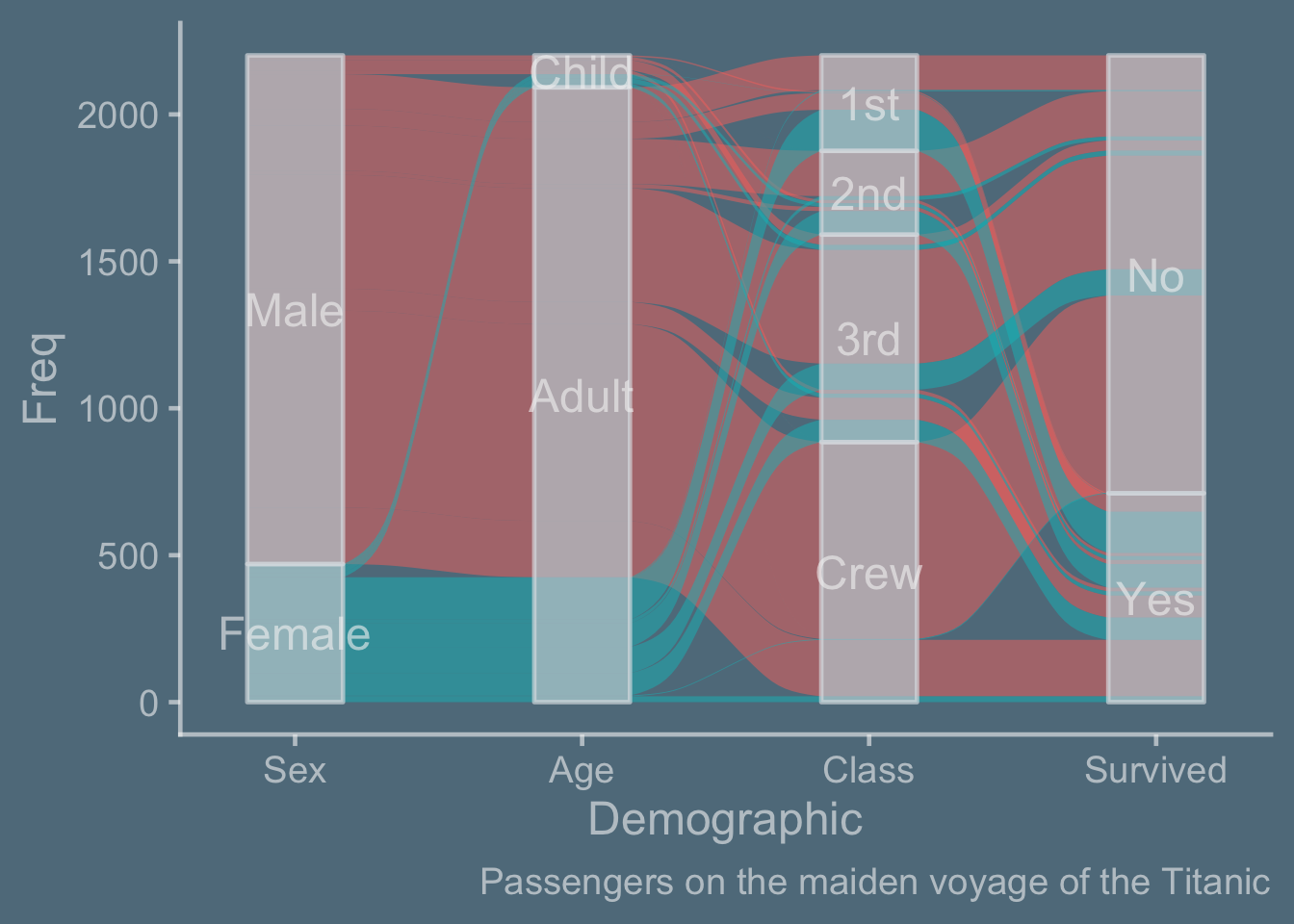
adding a caption , using labs(caption = "Passengers on the maiden voyage of the Titanic")

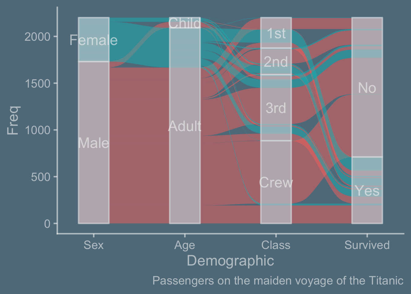
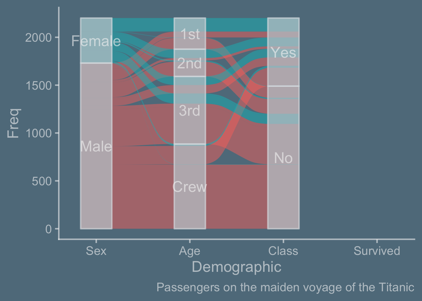
minimize flow crossing, using aes(axis1 = fct_rev(Sex))

minimize flow crossing, using aes(axis4 = fct_rev(Survived))

remove Age, using aes(axis2 = NULL)

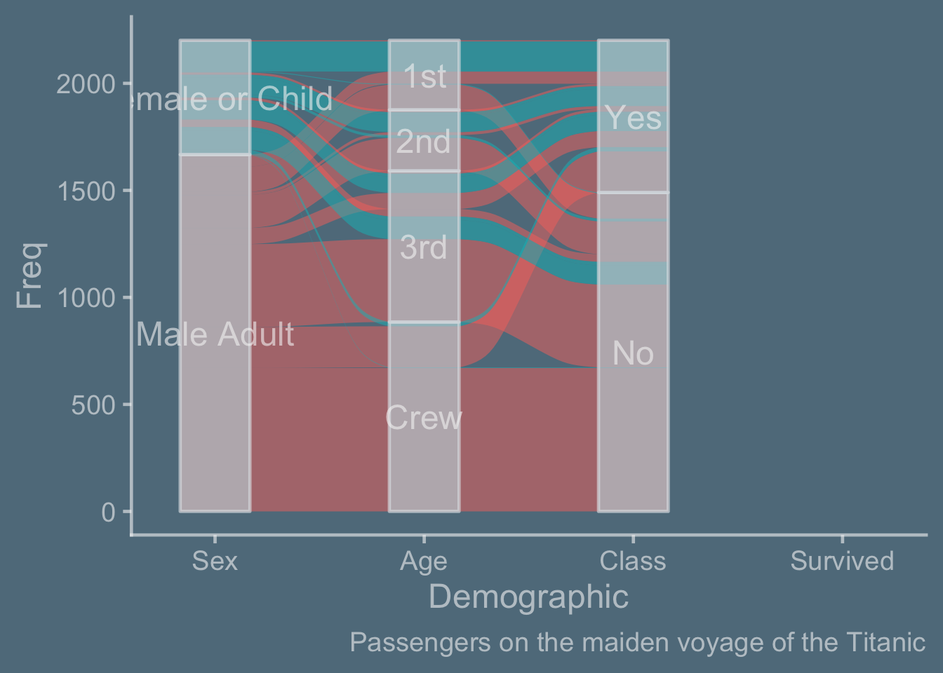
Replace axis 1, using aes(axis1 = ifelse(Sex == "Female" | Age == "Child", "Female or Child", "Male Adult"))

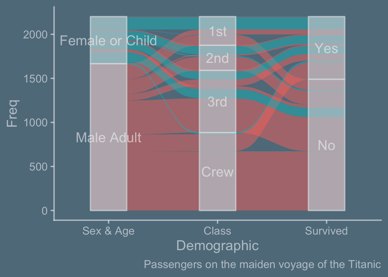
adjusting the x axis, using scale_x_discrete(limits = c("Sex & Age", "Class", "Survived"), expand = c(.2, .1))

More , using aes(fill = ifelse(Sex == "Female" | Age == "Child", "Female or Child", "Male Adult"))

  ggplot(data = titanic_wide) 

last_plot() +
    aes(y = Freq, axis1 = Sex, axis2 = Survived) 

last_plot() +
    ggchalkboard:::theme_slateboard(base_size = 18) 

last_plot() +
    geom_alluvium() 

last_plot() +
    geom_stratum(aes(fill = NULL)) 

last_plot() +
    geom_stratum_text() 

last_plot() +
    aes(axis1 = Age) 

last_plot() +
    aes(axis1 = Class) 

last_plot() +
    aes(axis1 = Age, axis2 = Class, axis3 = Survived) 

last_plot() +
    aes(axis1 = Sex, axis2 = Age, axis3 = Class, axis4 = Survived) 

last_plot() +
    aes(fill = Sex) 

last_plot() +
    guides(fill = "none") 

last_plot() +
    scale_x_discrete(limits = c("Sex", "Age", "Class", "Survived"), expand = c(.1, .1)) 

last_plot() +
    labs(x = "Demographic") 

last_plot() +
    labs(caption = "Passengers on the maiden voyage of the Titanic") 

last_plot() +
    aes(axis1 = fct_rev(Sex)) 

last_plot() +
    aes(axis4 = fct_rev(Survived)) 

last_plot() +
    aes(axis2 = NULL) 

last_plot() +
    aes(axis1 = ifelse(Sex == "Female" | Age == "Child", "Female or Child", "Male Adult")) 

last_plot() +
      scale_x_discrete(limits = c("Sex & Age", "Class", "Survived"), expand = c(.2, .1)) 

last_plot() +
    aes(fill = ifelse(Sex == "Female" | Age == "Child", "Female or Child", "Male Adult"))